9 Estadistica descriptiva

Vamos a usar la siguiente base de datos.

Cargamos librerias y leemos los datos

if (!require('findviews')) install.packages('findviews'); library('findviews')
if (!require('dplyr')) install.packages('dplyr'); library('dplyr')
if (!require('readr')) install.packages('readr'); library('readr')

if (!require('gt')) install.packages('gt'); library('gt')
if (!require('gtsummary')) install.packages('gtsummary'); library('gtsummary')


datos = read_csv(here::here("Data/07_Descriptive_statistics/Descriptive_statistics.csv")); datos

## # A tibble: 261 x 6
##       ID  Sexo  Edad Condition    VD  VD_t
##    <dbl> <dbl> <dbl> <chr>     <dbl> <dbl>
##  1     2     0    33 VI1          15  4893
##  2     2     0    33 VI1          15  9918
##  3     2     0    33 VI1          15   394
##  4     3     1    37 VI1           7  4099
##  5     3     1    37 VI1           7  6518
##  6     3     1    37 VI1           7   304
##  7     4     1    19 VI1          59  1792
##  8     4     1    19 VI1          59  9476
##  9     4     1    19 VI1          59   149
## 10     5     0    29 VI1          65  3280
## # … with 251 more rows

9.1 Gtsummaries

Para mas informacion y ejemplos de codigo: https://themockup.blog/posts/2020-09-04-10-table-rules-in-r/

Create a simple descriptive table:

gtsummary::tbl_summary(datos,
                       by = Sexo,
                       missing = "ifany") %>% 
  gtsummary::add_n()

## Warning: The `.dots` argument of `group_by()` is deprecated as of dplyr 1.0.0.

Characteristic	N	0, N = 99¹	1, N = 162¹
ID	261	11 (7, 26)	18 (12, 23)
Edad	261	23.0 (21.0, 33.0)	26.0 (21.0, 30.0)
Condition	261
VI1		33 (33%)	54 (33%)
VI2		33 (33%)	54 (33%)
VI3		33 (33%)	54 (33%)
VD	261	2 (1, 24)	3 (1, 43)
VD_t	261	1,265 (394, 4,546)	1,516 (369, 4,076)
¹ Median (IQR); n (%)

More complex:

Create a table for each Sex, combine the two and save to a file.

table1 = gtsummary::tbl_summary(datos %>% dplyr::filter(Sexo == 0) %>% dplyr::select(-Sexo),
                       by = Condition,
                       missing = "ifany",
                       type = list(Edad ~ 'categorical'),
                       statistic = list(Edad ~ "{n} ({p}%)")) %>% 
  gtsummary::add_n()


table2 = gtsummary::tbl_summary(datos %>% dplyr::filter(Sexo == 1) %>% dplyr::select(-Sexo),
                       by = Condition,
                       missing = "ifany",
                       type = list(Edad ~ 'categorical'),
                       statistic = list(Edad ~ "{n} ({p}%)")) %>% 
  gtsummary::add_n()


table_combined_Sexo = gtsummary::tbl_merge(list(table1, table2), tab_spanner = list("Females", "Males"))
table_combined_Sexo

Characteristic	Females				Males
Characteristic	N	VI1, N = 33¹	VI2, N = 33¹	VI3, N = 33¹	N	VI1, N = 54¹	VI2, N = 54¹	VI3, N = 54¹
ID	99	11 (7, 26)	11 (7, 26)	11 (7, 26)	162	18 (12, 23)	18 (12, 23)	18 (12, 23)
Edad	99				162
20		6 (18%)	6 (18%)	6 (18%)		6 (11%)	6 (11%)	6 (11%)
21		6 (18%)	6 (18%)	6 (18%)		3 (5.6%)	3 (5.6%)	3 (5.6%)
23		6 (18%)	6 (18%)	6 (18%)		6 (11%)	6 (11%)	6 (11%)
27		3 (9.1%)	3 (9.1%)	3 (9.1%)		3 (5.6%)	3 (5.6%)	3 (5.6%)
29		3 (9.1%)	3 (9.1%)	3 (9.1%)
33		3 (9.1%)	3 (9.1%)	3 (9.1%)
35		3 (9.1%)	3 (9.1%)	3 (9.1%)		3 (5.6%)	3 (5.6%)	3 (5.6%)
37		3 (9.1%)	3 (9.1%)	3 (9.1%)		3 (5.6%)	3 (5.6%)	3 (5.6%)
19						6 (11%)	6 (11%)	6 (11%)
22						3 (5.6%)	3 (5.6%)	3 (5.6%)
25						3 (5.6%)	3 (5.6%)	3 (5.6%)
28						9 (17%)	9 (17%)	9 (17%)
30						3 (5.6%)	3 (5.6%)	3 (5.6%)
32						3 (5.6%)	3 (5.6%)	3 (5.6%)
34						3 (5.6%)	3 (5.6%)	3 (5.6%)
VD	99	65 (24, 88)	2 (1, 4)	1 (0, 1)	162	66 (43, 72)	3 (1, 5)	1 (0, 1)
VD_t	99	1,265 (394, 4,546)	1,265 (394, 4,546)	1,265 (394, 4,546)	162	1,516 (377, 4,054)	1,516 (377, 4,054)	1,516 (377, 4,054)
¹ Median (IQR); n (%)

# Save table
gtsave(as_gt(table_combined_Sexo), file = here::here("Resultados/table-combined-bysex.png"))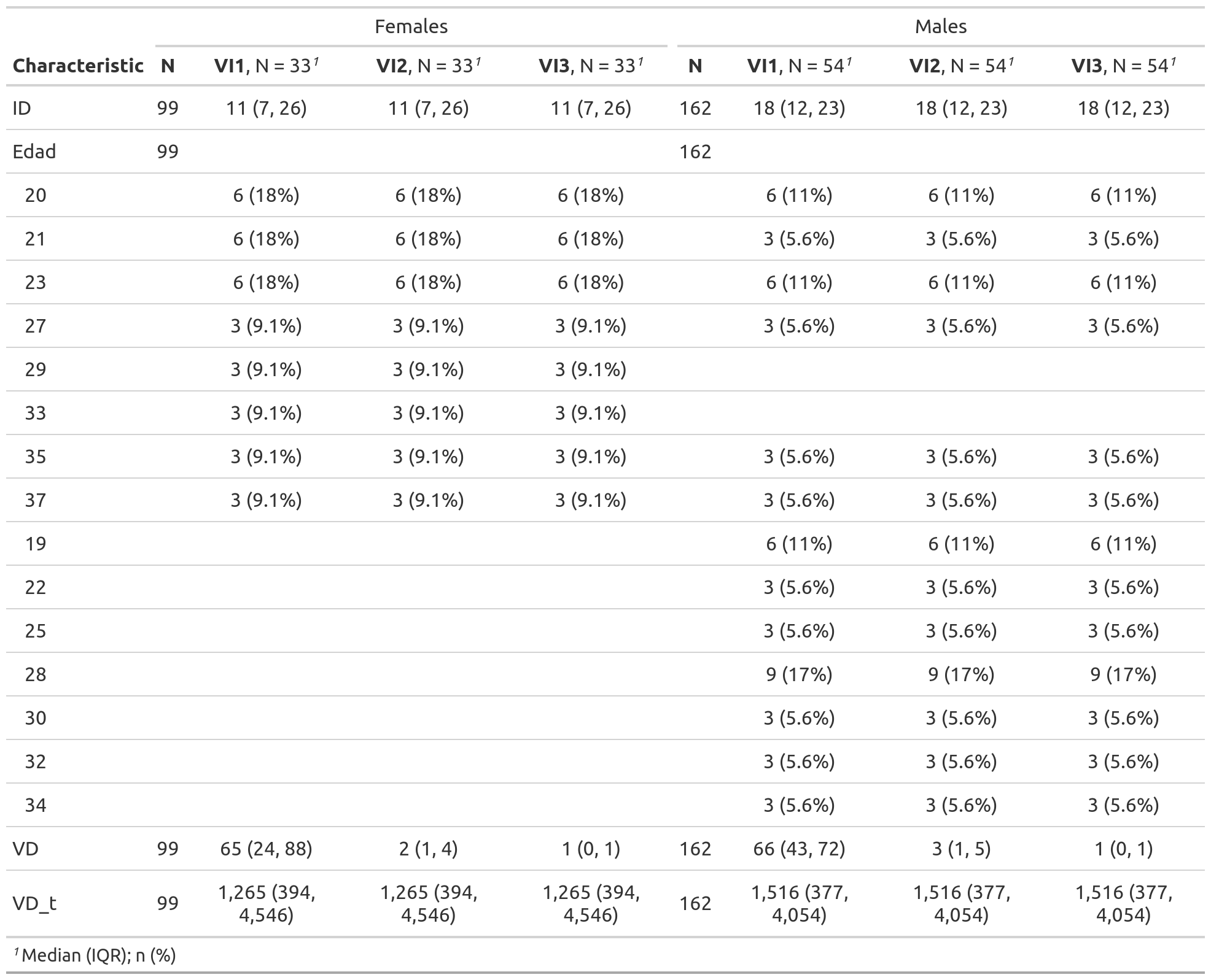

9.2 Summary de datos

# datos %>% group_by(Condition)  %>% summarise(VD = mean(VD), sd = sd(VD))
    
datos %>% 
  group_by(Condition) %>% 
  summarise(sd = sd(VD), VD = mean(VD))

##         sd       VD
## 1 31.20539 20.75862

# datos %>% filter(Edad > 18) %>% group_by(Condition, Sexo)  %>% summarise(VD = mean(VD), stdev = sd(VD), VD_t = mean(VD_t), num = length(VD))
    
datos %>% 
  filter(Edad > 18) %>%
  group_by(Condition, Sexo) %>%
  summarise(num = length(VD), stdev = sd(VD), VD = mean(VD), VD_t = mean(VD_t))

##   num    stdev       VD     VD_t
## 1 261 31.20539 20.75862 2554.149

# Todo en uno
datos %>%
  group_by(Condition) %>%
  summarise(num = length(VD), stdev = sd(VD), mean = mean(VD), max(VD), min(VD))

##   num    stdev     mean max(VD) min(VD)
## 1 261 31.20539 20.75862      99       0

9.2.1 Agrupamos por sujeto

datos %>%
  group_by(ID) %>%
  summarise(mean = mean(VD))

##       mean
## 1 20.75862

9.3 Descriptive tables latex

Using stargazer we can create tables showing summary statistics or a lm output. Here we use type = "html" to be able to show the table in this book. type = "latex" (default) shows the latex code.

if (!require('stargazer')) install.packages('stargazer'); library('stargazer')

## Loading required package: stargazer

## 
## Please cite as:

##  Hlavac, Marek (2018). stargazer: Well-Formatted Regression and Summary Statistics Tables.

##  R package version 5.2.2. https://CRAN.R-project.org/package=stargazer

stargazer(datos %>% as.data.frame(), type="html")


Statistic	N	Mean	St. Dev.	Min	Pctl(25)	Pctl(75)	Max

ID	261	16.000	8.383	2	9	23	30
Sexo	261	0.621	0.486	0	0	1	1
Edad	261	26.207	5.767	19	21	30	37
VD	261	20.759	31.205	0	1	41	99
VD_t	261	2,554.149	2,702.144	13	380	4,099	9,918

9.4 Visualize missing values

With Amelia

if (!require('Amelia')) install.packages('Amelia'); library('Amelia')

## Loading required package: Amelia

## Loading required package: Rcpp

## ## 
## ## Amelia II: Multiple Imputation
## ## (Version 1.7.6, built: 2019-11-24)
## ## Copyright (C) 2005-2021 James Honaker, Gary King and Matthew Blackwell
## ## Refer to http://gking.harvard.edu/amelia/ for more information
## ##

datos = datos %>% mutate(Sexo = ifelse(Edad == 37, NA, Sexo))

missmap(datos)

## Warning: Unknown or uninitialised column: `arguments`.

## Warning: Unknown or uninitialised column: `arguments`.

## Warning: Unknown or uninitialised column: `imputations`.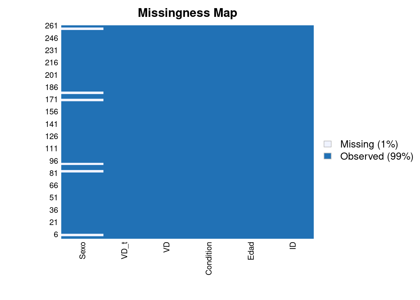

With ggplot and reshape2

# With ggplot
# A function that plots missingness
if (!require('reshape2')) install.packages('reshape2'); library('reshape2')
if (!require('ggplot2')) install.packages('ggplot2'); library('ggplot2')

ggplot_missing <- function(x){
  
  x %>% 
    is.na %>%
    melt %>%
    ggplot(data = .,
           aes(x = Var2,
               y = Var1)) +
    geom_raster(aes(fill = value)) +
    scale_fill_grey(name = "",
                    labels = c("Present","Missing")) +
    theme_minimal() + 
    theme(axis.text.x  = element_text(angle=45, vjust=0.5)) + 
    labs(x = "Variables in Dataset",
         y = "Rows / observations")
}

ggplot_missing(datos)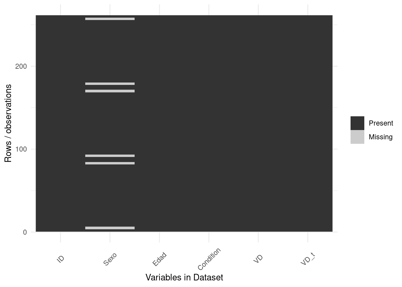

if (!require('naniar')) install.packages('naniar'); library('naniar')

## Loading required package: naniar

# Add some missing in Edad
set.seed(10)
missing = rbinom(261, 1, 0.3)
datos$Edad = with(datos, ifelse(Edad >= 30 & missing == 1, NA, Edad))

# Visualize upset plot
  # Missing in Edad, Missing in Sexo, Missing in Sexo AND Edad
datos %>% 
  gg_miss_upset()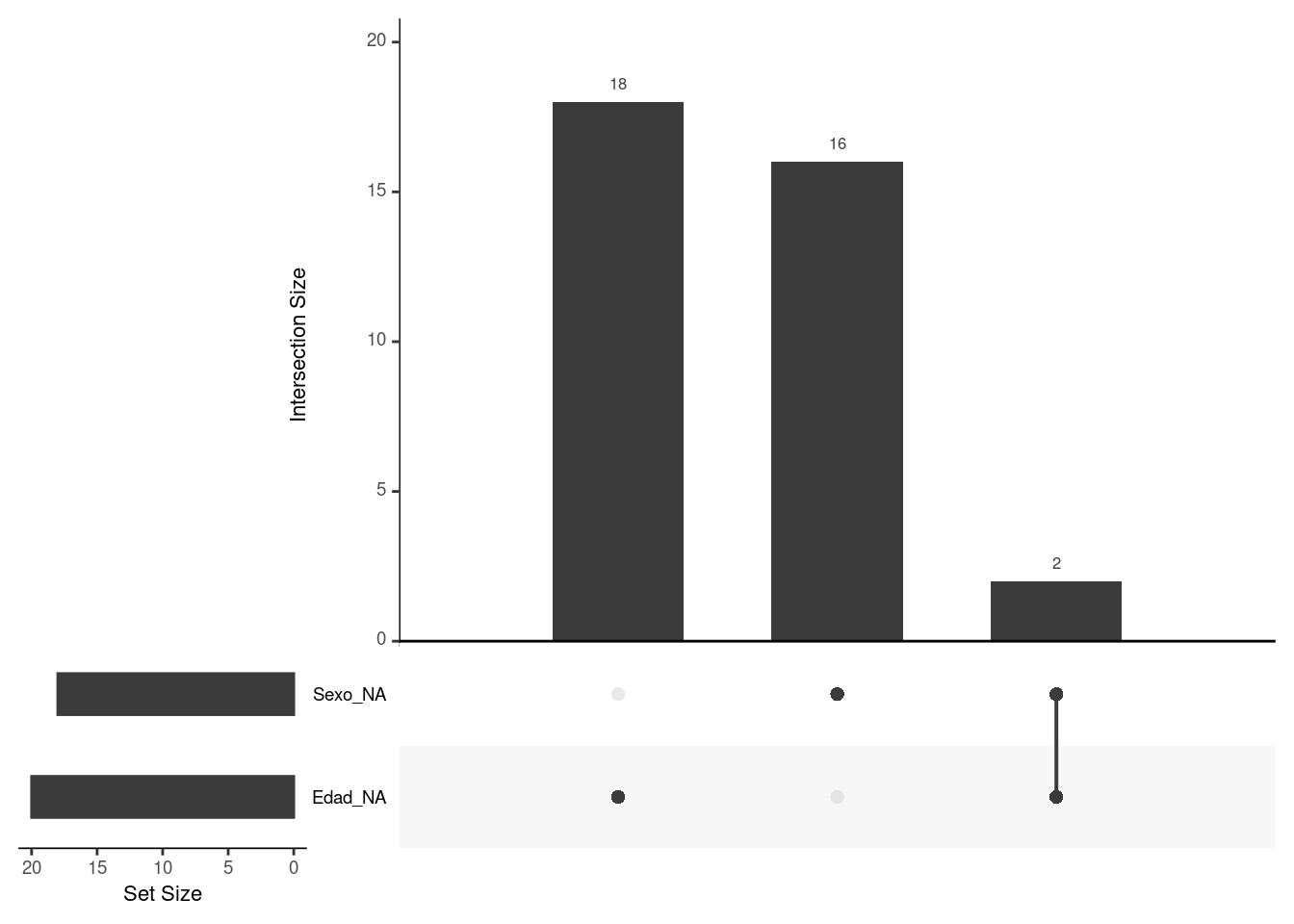

9.5 Tutorial externo

Tutorial para colapsar datos

9.6 Findviews

Lanzar el siguiente comando para explorar visualmente los datos:

´findviews(datos)´

Ver pagina en Github