10 Estadistica inferencial

WIP: REVISAR PAQUETE AFEX

Permite definir variables intra y entre… y sacar posthocs!
https://cran.r-project.org/web/packages/afex/afex.pdf

a = aov_ez(“ID,” “VD,” datos_long, within = c(“VI1,” “VI2,” “VI3”))

lsmip(a, VI1 ~ VI2 * VI3)

lsmeans(a, “VI1,” contr = “pairwise”) lsmeans(a, “VI2,” contr = “pairwise”) lsmeans(a, “VI3,” contr = “pairwise”)

lsmeans(a, c(“VI1,” “VI2,” “VI3”), contr = “pairwise”)

Why Psychologists Should Always Report the W-test Instead of the F-Test ANOVA https://psyarxiv.com/wnezg

WIP: REVISAR

http://www.quantide.com/raccoon-ch-2-4-3-way-anova/
Don’t do balance tests: http://janhove.github.io/reporting/2014/09/26/balance-tests

Luego de tener algo parecido a una base de datos ordenada, y haber examinado y vizualizado nuestros datos, es posible que quieras analizarlos.

Para esto aprenderemos algo sobre la lógica de contrucción de modelos y formulas con los cuales podremos armar varias de las pruebas estadísticas clásicas y facilitara la comprensión de otras funciones más complejas como las relacionadas a Modelos re regresión más complejos y Modelos de Ecuaciones Estructurales.

##Algo sobre Modelos y Fórmulas En terminos sencillos, un modelo es una conjetura sobre que tipo de relación tienen las variables en juego.

Por ejemplo yo podria suponer que a medida que aumenta el consumo de alcohol, nuestra percepción de belleza decae.

R tiene sencillas fórmulas para representar este tipo de relaciones.

Si nosotros pensamos que el consumo Alcohol predice el Atractivo de la persona con la que filteamos, podemos formularlo como un modelo de la forma:

#fórmula básica
formula = "Atractivo ~ Alcohol"

Si además pensamos que el Sexo tambien puede ser un predictor, modificamos el modelo inicial:

#añadir variables predictoras
formula = "Atractivo ~ Alcohol + Sexo"

En el caso de que 2 variables, Alcohol y Sexo sean predictores, es posible pensar que estas pueden interaccionas. Podemos agregar la interación de varias formas:

#versión extendida
formula = "Atractivo ~ Alcohol + Sexo + Alcohol*Sexo"

#versión corta
formula = "Atractivo ~ Alcohol*Sexo"

En resumen, todo lo que esta a la derecha del simbolo ~ es considerado un predictor o variable independiente, y todo lo que esta a la izquierda es una variable de resultado o una variable dependiente. No utilizamos el simbolo =, <- o == ya que no estamos ni asignando ni haciendo una equivalencia lógica, y podriamos confundir a R.

Existen casos (por ejemplo, correlación o chi-cuadrado) en donde no hay una predicción propiamente tal. En estos casos se elimina del modelo la variable de resultado:

#fórmula para modelo sin predictor o asociativo
formula = "~ Atractivo + Alcohol"

##Preparación de datos y packages

Para muchos de los análisis que vienen a continuación hemos creado una base de datos, la cual puedes descargar Aquí.

#Packages
if (!require('readr')) install.packages('readr'); library('readr')
if (!require('dplyr')) install.packages('dplyr'); library('dplyr')
if (!require('yarrr')) install.packages('yarrr'); library('yarrr')
if (!require('car')) install.packages('car'); library('car')

## Loading required package: car

## Loading required package: carData

## 
## Attaching package: 'car'

## The following object is masked from 'package:psych':
## 
##     logit

## The following object is masked from 'package:dplyr':
## 
##     recode

## The following object is masked from 'package:purrr':
## 
##     some

#Importar dataframe
df = read_csv("Data/08-Data_analysis/ANOVA_1.csv")

## 
## ── Column specification ────────────────────────────────────────────────────────
## cols(
##   Id = col_double(),
##   AccuracyIz = col_double(),
##   Moral = col_double(),
##   Tom = col_double(),
##   Empatia = col_double(),
##   Sexo = col_double(),
##   Edad = col_double(),
##   AccuracyDer = col_double(),
##   AdapSoc = col_double(),
##   FunEjec = col_double()
## )

#Muestra las primeras 10 observaciones
df

## # A tibble: 237 x 10
##       Id AccuracyIz Moral   Tom Empatia  Sexo  Edad AccuracyDer AdapSoc FunEjec
##    <dbl>      <dbl> <dbl> <dbl>   <dbl> <dbl> <dbl>       <dbl>   <dbl>   <dbl>
##  1     1         34     1    29      63     0    62          13      40      25
##  2     2         13    NA    23      55     0    53           8      43     175
##  3     3         20     1    26      27     0    18          14      38      18
##  4     4         24     1    21      33     0    40          14      48      16
##  5     5         20     1    18      35     1    65          15      48     175
##  6     6          2     0    23      38    NA    NA          12      35     205
##  7     7         13     1    19      38     0    56           5      16       8
##  8     8         27     1    15      42     1    70           8      41      21
##  9     9         37     1    23      36     0    43          23      38      26
## 10    10         27     0    20      51     1    52           9      24       8
## # … with 227 more rows

#Recodificar variable sexo de numérico a factor con etiquetas
df = df %>% mutate(Sexo = ifelse(Sexo == 0, "mujer", "hombre")) %>% mutate(Sexo = as.factor(Sexo))

##Prueba t para muestras independientes

###Contando la historia… Evaluación de diferencias por Sexo en una prueba de Teoría de la mente Tom

###Test

#En primer lugar comprobamos el supuesto de homogeneidad de varianzas

#levene test {car} para homogeneidad de las varianzas
leveneTest(df$Tom ~ df$Sexo)

## Levene's Test for Homogeneity of Variance (center = median)
##        Df F value Pr(>F)
## group   1  0.7558 0.3856
##       228

#Ingresamos nuestro modelo en la función t.test()
t.test(Tom ~ Sexo, df,  var.equal = T, paired = F)

## 
##  Two Sample t-test
## 
## data:  Tom by Sexo
## t = -2.4618, df = 228, p-value = 0.01456
## alternative hypothesis: true difference in means is not equal to 0
## 95 percent confidence interval:
##  -2.6763463 -0.2967329
## sample estimates:
## mean in group hombre  mean in group mujer 
##             21.28070             22.76724

#Reporte descriptivo y Vizualización
df %>% 
  na.omit(Tom) %>% 
  group_by(Sexo) %>% 
  summarise(mean = mean(Tom), sd = sd(Tom))

##       mean       sd
## 1 22.11574 4.495014

pirateplot(Tom ~ Sexo, 
           data = df, 
           ylim = c(0, 40), 
           xlab = "Metodo", 
           ylab = "Nota", 
           main = "t test Pirateplot", 
           point.pch = 16, 
           pal = "basel")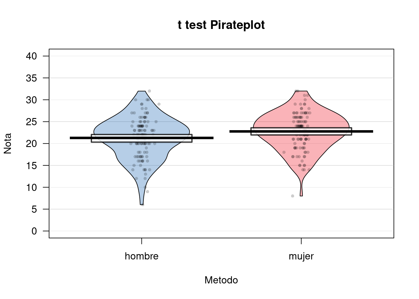

##Prueba t para muestras dependientes

###Contando la historia… En una tarea de disparo a objetivos, queremos evaluar si existen diferencias en la precisión de los sujetos a objetivos que aparecen a la Izquierda (AccuracyIz) o a la Derecha (AccuracyDer) del monitor.

###Test

#Ingresamos nuestro modelo en la función t.test()
t.test(df$AccuracyIz, df$AccuracyDer, paired = T)

## 
##  Paired t-test
## 
## data:  df$AccuracyIz and df$AccuracyDer
## t = 22.904, df = 233, p-value < 2.2e-16
## alternative hypothesis: true difference in means is not equal to 0
## 95 percent confidence interval:
##  10.05377 11.94623
## sample estimates:
## mean of the differences 
##                      11

##Correlación de Pearson

###Contando la historia… Se desea evaluar si existe alguna relación entre Teoria de la Mente (Tom) y el grado de Empatía de los sujetos (Empatia).

###Test

#Correlación de Pearson
cor.test(~ Tom + Empatia, data = df)

## 
##  Pearson's product-moment correlation
## 
## data:  Tom and Empatia
## t = 1.9789, df = 229, p-value = 0.04903
## alternative hypothesis: true correlation is not equal to 0
## 95 percent confidence interval:
##  0.0005956093 0.2544818239
## sample estimates:
##       cor 
## 0.1296633

#Visualizar Diagrama de Dispersión
ggplot(df, aes(Tom, Empatia)) +
  theme_bw() +
  geom_point(shape = 16, col = transparent("red", .4))

## Warning: Removed 6 rows containing missing values (geom_point).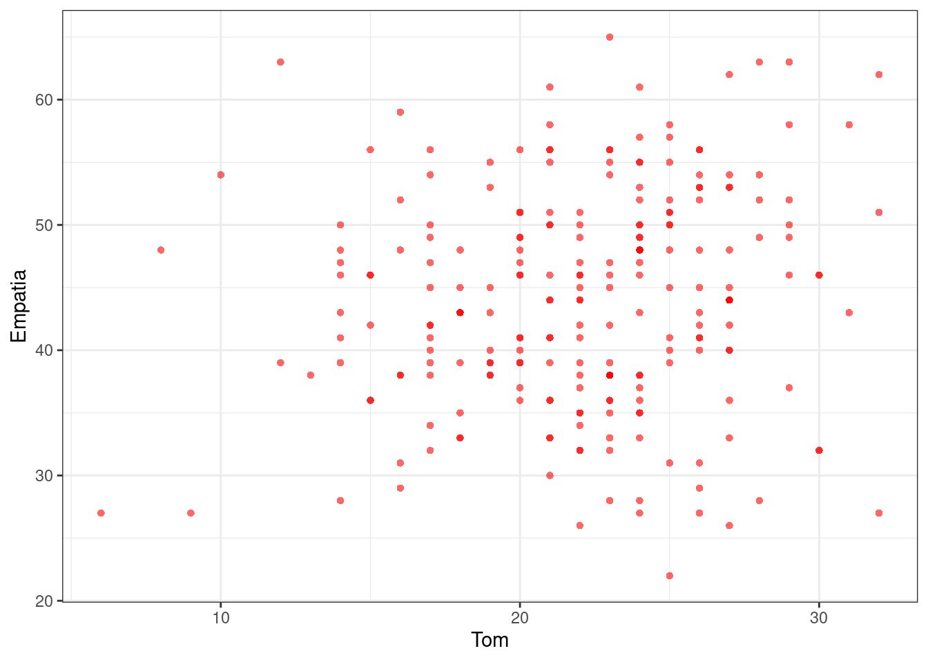

#Selecione un subconjunto de variables para la correlación multiple
cordata = df %>% dplyr::select(-Id,-Moral,-Sexo,-AccuracyIz,-AccuracyDer,-Edad)

#carga libreria Hmisc
if (!require('Hmisc')) install.packages('Hmisc'); library('Hmisc')

## Loading required package: Hmisc

## Loading required package: survival

## Loading required package: Formula

## 
## Attaching package: 'Hmisc'

## The following object is masked from 'package:gt':
## 
##     html

## The following objects are masked from 'package:plyr':
## 
##     is.discrete, summarize

## The following object is masked from 'package:psych':
## 
##     describe

## The following objects are masked from 'package:dplyr':
## 
##     src, summarize

## The following objects are masked from 'package:base':
## 
##     format.pval, units

#correlación multiple
rcorr(as.matrix(cordata), type = "pearson")

##          Tom Empatia AdapSoc FunEjec
## Tom     1.00    0.13    0.16    0.10
## Empatia 0.13    1.00    0.25    0.06
## AdapSoc 0.16    0.25    1.00    0.15
## FunEjec 0.10    0.06    0.15    1.00
## 
## n
##         Tom Empatia AdapSoc FunEjec
## Tom     232     231     226     231
## Empatia 231     235     229     234
## AdapSoc 226     229     231     230
## FunEjec 231     234     230     236
## 
## P
##         Tom    Empatia AdapSoc FunEjec
## Tom            0.0490  0.0130  0.1331 
## Empatia 0.0490         0.0001  0.3760 
## AdapSoc 0.0130 0.0001          0.0204 
## FunEjec 0.1331 0.3760  0.0204

##Regresión Simple

###Contando la historia…

Evaluaremos como las Funciones ejecutivas (FunEjec) pueden predecir la Precisión a objetivos en una tarea atencional (Accuracy).

Para esto primero añadiremos una nueva variable Accuracy la cual será el promedio de precisión para los objetivos Derechos (AccuracyDer) e Izquierdos (AccuracyIz). Lo realizaremos con la función mutate antes revisada en el apartado de manipulación de datos.

Además filtraremos a los sujetos con puntajes bajos (menos de 50 puntos).

#Creamos nueva variable "Accuracy" con la función mutate() {dplyr}
df = df %>% mutate(Accuracy = (AccuracyIz + AccuracyDer)/2)

#Utilizar observaciones con puntajes de Funcion ejecutiva sobre 50 puntos.
df = df %>% filter(FunEjec > 50)

###Test

#Insertamos nuestra fórmula al Modelo de Regresión Simple
fit = lm(Accuracy ~ FunEjec, df)

#Resumen de Coeficientes y Parametros del modelo
summary(fit)

## 
## Call:
## lm(formula = Accuracy ~ FunEjec, data = df)
## 
## Residuals:
##     Min      1Q  Median      3Q     Max 
## -11.587  -3.087   0.413   2.163  10.038 
## 
## Coefficients:
##             Estimate Std. Error t value Pr(>|t|)    
## (Intercept)  5.76939    2.83753   2.033   0.0457 *  
## FunEjec      0.06252    0.01457   4.292 5.36e-05 ***
## ---
## Signif. codes:  0 '***' 0.001 '**' 0.01 '*' 0.05 '.' 0.1 ' ' 1
## 
## Residual standard error: 4.729 on 73 degrees of freedom
##   (2 observations deleted due to missingness)
## Multiple R-squared:  0.2015, Adjusted R-squared:  0.1905 
## F-statistic: 18.42 on 1 and 73 DF,  p-value: 5.363e-05

#Intevalos de Confianza de los parámetros del modelo
confint(fit, level = 0.95)

##                  2.5 %      97.5 %
## (Intercept) 0.11419463 11.42458615
## FunEjec     0.03349037  0.09155961

#Visualizar Diagrama de Dispersión para Regresión
ggplot(df, aes(FunEjec, Accuracy)) +
  theme_bw() +
  geom_point(shape = 16, col = transparent("black", .4)) + 
  geom_smooth(method = lm , color = "red", se = T)

## `geom_smooth()` using formula 'y ~ x'

## Warning: Removed 2 rows containing non-finite values (stat_smooth).

## Warning: Removed 2 rows containing missing values (geom_point).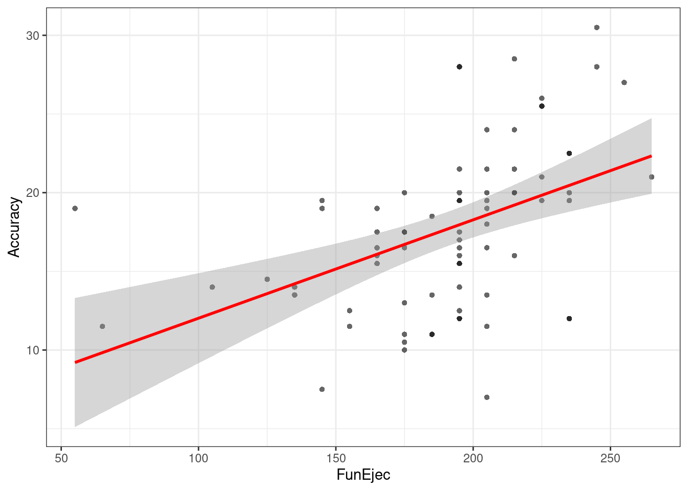

##Análsis de la Varianza (1 Factor) Esta vez trabajaremos con otra base de datos, la cual puedes descargar Aquí. Se recomienda en esta oportunidad limpiar nuestro espacio de trabajo. Para esto podemos presionar Ctrl + Shift + F10 o utilizar la función:

rm(list=ls())

###Preparación de datos y packages

#Packages
if (!require('readr')) install.packages('readr'); library('readr')
if (!require('dplyr')) install.packages('dplyr'); library('dplyr')
if (!require('stats')) install.packages('stats'); library('stats')
if (!require('car')) install.packages('car'); library('car')
if (!require('apaTables')) install.packages('apaTables'); library('apaTables')

## Loading required package: apaTables

#Importar dataframe
df = read_csv("Data/08-Data_analysis/ANOVA_2.csv")

## 
## ── Column specification ────────────────────────────────────────────────────────
## cols(
##   Metodo = col_double(),
##   Nota = col_double()
## )

#Muestra las primeras 10 observaciones
df

## # A tibble: 30 x 2
##    Metodo  Nota
##     <dbl> <dbl>
##  1      1    50
##  2      1    45
##  3      1    48
##  4      1    47
##  5      1    45
##  6      1    49
##  7      1    50
##  8      1    54
##  9      1    57
## 10      1    55
## # … with 20 more rows

#Recodificar variable Metodo de numérico a factor con etiquetas
df = df %>% mutate(Metodo = ifelse(Metodo == 1, "Electroshock", ifelse(Metodo == 2, "Indiferencia", "Buen trabajo"))) %>% mutate(Metodo = as.factor(Metodo))

###Contando la historia… Se desea evaluar que métodos pueden contribuir (o no) al aprendizaje de estadísticas en R. Para esto tenemos las variables Metodo (si se uso Electroshock, la fria Indiferencia o un “Buen trabajo!”) y la Nota nota que se obtuvo en el curso.

###Test

#Introducimos la formula al Modelo con la función de ANOVA aov()
fit = aov(Nota ~ Metodo, df)

#Summario de Parámetros y Coeficientes
summary(fit)

##             Df Sum Sq Mean Sq F value   Pr(>F)    
## Metodo       2 1205.1   602.5   21.01 3.15e-06 ***
## Residuals   27  774.4    28.7                     
## ---
## Signif. codes:  0 '***' 0.001 '**' 0.01 '*' 0.05 '.' 0.1 ' ' 1

#levene test {car} para homogeneidad de las varianzas
leveneTest(df$Nota ~ df$Metodo)

## Levene's Test for Homogeneity of Variance (center = median)
##       Df F value Pr(>F)
## group  2  1.7343 0.1956
##       27

#Comparaciones Multiples mediante función TukeyHSD() {stats}
TukeyHSD(fit)

##   Tukey multiple comparisons of means
##     95% family-wise confidence level
## 
## Fit: aov(formula = Nota ~ Metodo, data = df)
## 
## $Metodo
##                            diff          lwr       upr     p adj
## Electroshock-Buen trabajo -15.4 -21.33834579 -9.461654 0.0000020
## Indiferencia-Buen trabajo  -9.4 -15.33834579 -3.461654 0.0015175
## Indiferencia-Electroshock   6.0   0.06165421 11.938346 0.0472996

#Reporte descriptivo y Vizualización
df %>% 
  group_by(Metodo) %>% 
  summarise(mean = mean(Nota), sd = sd(Nota))

##       mean       sd
## 1 57.13333 8.261808

pirateplot(Nota ~ Metodo, 
           data = df, 
           ylim = c(0, 100), 
           xlab = "Metodo", 
           ylab = "Nota", 
           main = "ANOVA Pirateplot", 
           point.pch = 16, 
           pal = "basel")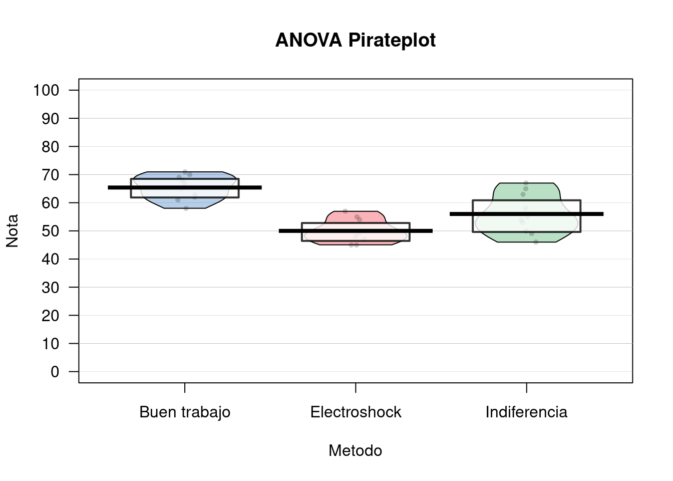

###Tablas

apa.1way.table(iv = Metodo, dv = Nota, data = df, filename = "Resultados/Figure1_APA.doc", table.number = 1)

## 
## 
## Table 1 
## 
## Descriptive statistics for Nota as a function of Metodo.  
## 
##        Metodo     M   SD
##  Buen trabajo 65.40 4.30
##  Electroshock 50.00 4.14
##  Indiferencia 56.00 7.10
## 
## Note. M and SD represent mean and standard deviation, respectively.
##

apa.aov.table(fit, filename = "Resultados/Figure2_APA.doc",table.number = 2)

## 
## 
## Table 2 
## 
## ANOVA results using Nota as the dependent variable
##  
## 
##    Predictor       SS df       MS       F    p partial_eta2 CI_90_partial_eta2
##  (Intercept) 42771.60  1 42771.60 1491.26 .000                                
##       Metodo  1205.07  2   602.53   21.01 .000          .61         [.36, .71]
##        Error   774.40 27    28.68                                             
## 
## Note: Values in square brackets indicate the bounds of the 90% confidence interval for partial eta-squared

##Análsis de la Varianza (2 Factores)

###Descarga

Esta vez nuevamente trabajaremos con otra base de datos, la cual puedes descargar Aquí. Se recomienda nuevamente limpiar nuestro espacio de trabajo. Para esto podemos presionar Ctrl + Shift + F10 o utilizar la función:

rm(list = ls())

###Preparación de datos y packages

#Packages
if (!require('readr')) install.packages('readr'); library('readr')
if (!require('dplyr')) install.packages('dplyr'); library('dplyr')
if (!require('stats')) install.packages('stats'); library('stats')
if (!require('car')) install.packages('car'); library('car')



#Importar dataframe
df = read_csv("Data/08-Data_analysis/ANOVA_3.csv")

## 
## ── Column specification ────────────────────────────────────────────────────────
## cols(
##   Sexo = col_double(),
##   Alcohol = col_double(),
##   Atractivo = col_double()
## )

#Muestra las primeras 10 observaciones
df

## # A tibble: 32 x 3
##     Sexo Alcohol Atractivo
##    <dbl>   <dbl>     <dbl>
##  1     1       0        65
##  2     1       0        70
##  3     1       0        60
##  4     1       0        60
##  5     1       0        60
##  6     1       0        55
##  7     1       0        60
##  8     1       0        55
##  9     1       1        55
## 10     1       1        65
## # … with 22 more rows

#Recodificar variable Sexo y Alcohol de numérico a factor con etiquetas
df = df %>% mutate(Sexo = ifelse(Sexo == 0, "mujer", "hombre")) %>% mutate(Sexo = as.factor(Sexo))
df = df %>% mutate(Alcohol = ifelse(Alcohol == 0, "No consume", "Tres Shop")) %>% mutate(Alcohol = as.factor(Alcohol))

###Contando la historia… A veces cuando bebemos bebidas espirituosas, podemos sobreestimar el atractivo de otras personas. Esto en psicología lo conocemos como “Beer Glass Effect.” Deseamos ver este efecto, pero además ver si el Sexo influye también.

Para esto tenemos las variables Alcohol (Si ha bebido o no), el Sexo del bebedor y la puntuación de Atractivo de la persona con la que flirtea aquella noche.

###Test

#Ajustamos el modelo con la funcion de ANOVA aov()
fit = aov(Atractivo ~ Sexo * Alcohol, df)

#Summario de Parámetros y Coeficientes
summary(fit)

##              Df Sum Sq Mean Sq F value   Pr(>F)    
## Sexo          1  488.3   488.3    6.54   0.0163 *  
## Alcohol       1 2363.3  2363.3   31.65 5.03e-06 ***
## Sexo:Alcohol  1 1582.0  1582.0   21.19 8.20e-05 ***
## Residuals    28 2090.6    74.7                     
## ---
## Signif. codes:  0 '***' 0.001 '**' 0.01 '*' 0.05 '.' 0.1 ' ' 1

#Comparaciones Multiples mediante función TukeyHSD() {stats}
TukeyHSD(fit)

##   Tukey multiple comparisons of means
##     95% family-wise confidence level
## 
## Fit: aov(formula = Atractivo ~ Sexo * Alcohol, data = df)
## 
## $Sexo
##                 diff       lwr       upr     p adj
## mujer-hombre -7.8125 -14.07042 -1.554575 0.0162548
## 
## $Alcohol
##                          diff       lwr       upr p adj
## Tres Shop-No consume -17.1875 -23.44542 -10.92958 5e-06
## 
## $`Sexo:Alcohol`
##                                       diff        lwr        upr     p adj
## mujer:No consume-hombre:No consume   6.250  -5.546177  18.046177 0.4820693
## hombre:Tres Shop-hombre:No consume  -3.125 -14.921177   8.671177 0.8869596
## mujer:Tres Shop-hombre:No consume  -25.000 -36.796177 -13.203823 0.0000186
## hombre:Tres Shop-mujer:No consume   -9.375 -21.171177   2.421177 0.1564908
## mujer:Tres Shop-mujer:No consume   -31.250 -43.046177 -19.453823 0.0000004
## mujer:Tres Shop-hombre:Tres Shop   -21.875 -33.671177 -10.078823 0.0001309

#Reporte descriptivo y Vizualización
df %>% 
  group_by(Alcohol,Sexo) %>% 
  summarise(mean = mean(Atractivo), sd = sd(Atractivo))

##       mean       sd
## 1 55.15625 14.50719

df %>% 
  group_by(Alcohol) %>% 
  summarise(mean = mean(Atractivo), sd = sd(Atractivo))

##       mean       sd
## 1 55.15625 14.50719

df %>% 
  group_by(Sexo) %>% 
  summarise(mean = mean(Atractivo), sd = sd(Atractivo))

##       mean       sd
## 1 55.15625 14.50719

pirateplot(Atractivo ~ Sexo + Alcohol, 
           data = df, 
           ylim = c(0, 100), 
           xlab = "Sex*Alcohol", 
           ylab = "Attractiveness Score", 
           main = "ANOVA Pirateplot", 
           point.pch = 16, 
           pal = "basel")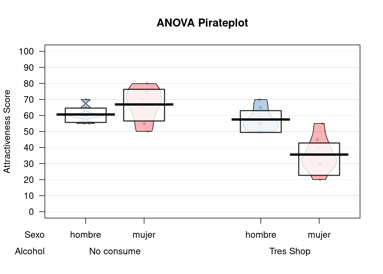

###Tablas

apa.2way.table(iv1 = Sexo, iv2 = Alcohol, dv = Atractivo, data = df, filename = "Resultados/Figure3_APA.doc", table.number = 3)

## 
## 
## Table 3 
## 
## Means and standard deviations for Atractivo as a function of a 2(Sexo) X 2(Alcohol) design 
## 
##            Alcohol                      
##         No consume       Tres Shop      
##    Sexo          M    SD         M    SD
##  hombre      60.62  4.96     57.50  7.07
##   mujer      66.88 10.33     35.62 10.84
## 
## Note. M and SD represent mean and standard deviation, respectively.

apa.aov.table(fit, filename = "Resultados/Figure4_APA.doc",table.number = 4)

## 
## 
## Table 4 
## 
## ANOVA results using Atractivo as the dependent variable
##  
## 
##       Predictor       SS df       MS      F    p partial_eta2
##     (Intercept) 29403.12  1 29403.12 393.80 .000             
##            Sexo   156.25  1   156.25   2.09 .159          .07
##         Alcohol    39.06  1    39.06   0.52 .475          .02
##  Sexo x Alcohol  1582.03  1  1582.03  21.19 .000          .43
##           Error  2090.62 28    74.66                         
##  CI_90_partial_eta2
##                    
##          [.00, .24]
##          [.00, .16]
##          [.19, .58]
##                    
## 
## Note: Values in square brackets indicate the bounds of the 90% confidence interval for partial eta-squared

10.1 Referencias y Fuentes

10.2 Association test

A.K.A. X square test of independence

WIP - Alternatives

# Con datos de estudio Merlin
# prop.test(table(DB_all$Ahorro_Dico, DB_all$Futuro_d))
# chisq.test(table(DB_all$Ahorro_Dico, DB_all$Futuro_d))

# # More powerful
# Exact::exact.test(table(DB_all$Ahorro_Dico, DB_all$Futuro_d))
# BayesFactor::contingencyTableBF(table(DB_all$Ahorro_Dico, DB_all$Futuro_d), sampleType = "indepMulti", fixedMargin = "rows")

Libraries

if (!require('BayesFactor')) install.packages('BayesFactor'); library('BayesFactor')
if (!require('lsr')) install.packages('lsr'); library('lsr')

Import data - WIP We use the following dataset.

#Import to variable "dataset"
dataset = read.csv("Data/08-Data_analysis/Association_test.csv")

#Show first 5 rows
head(dataset)

##    X    ID Dem_Gender Dem_Age Dem_Education       SET    answer   Time Formato
## 1  4 71827          2      34             4 Resp_SET1 0.3333333 12.905      FN
## 2  5  1946          1      29             6 Resp_SET1 0.3333333 38.895      FN
## 3  6 83294          2      25             6 Resp_SET1 0.3333333 42.473      FN
## 4  8 34065          1      29             6 Resp_SET1 0.6666667 16.438      PR
## 5  9 39707          1      30             5 Resp_SET1 0.3333333 60.794      PR
## 6 10 69772          2      28             2 Resp_SET1 0.5000000 26.169      PR
##   Problema Accuracy      Error Accuracy_factor Formato_factor Problema_factor
## 1   DECIMA        1  0.0000000               1             FN          DECIMA
## 2   DECIMA        1  0.0000000               1             FN          DECIMA
## 3   UNIDAD        1  0.0000000               1             FN          UNIDAD
## 4   UNIDAD        0 -0.3333333               0             PR          UNIDAD
## 5   DECIMA        1  0.0000000               1             PR          DECIMA
## 6   UNIDAD        0 -0.1666667               0             PR          UNIDAD
##   Time_set1
## 1    12.905
## 2    38.895
## 3    42.473
## 4    16.438
## 5    60.794
## 6    26.169

Prepare data

# Convert to factors
dataset$Accuracy_factor = as.factor(dataset$Accuracy)
dataset$Formato_factor = as.factor(dataset$Formato)
dataset$Problema_factor = as.factor(dataset$Problema)

10.2.1 Frequentist¹

# Accuracy_factor + Formato_factor
crosstab_Formato <- xtabs(~ Accuracy_factor + Formato_factor, dataset); crosstab_Formato

##                Formato_factor
## Accuracy_factor FN PR
##               0 18 24
##               1 66 57

associationTest(formula = ~ Accuracy_factor + Formato_factor, data = dataset )

## 
##      Chi-square test of categorical association
## 
## Variables:   Accuracy_factor, Formato_factor 
## 
## Hypotheses: 
##    null:        variables are independent of one another
##    alternative: some contingency exists between variables
## 
## Observed contingency table:
##                Formato_factor
## Accuracy_factor FN PR
##               0 18 24
##               1 66 57
## 
## Expected contingency table under the null hypothesis:
##                Formato_factor
## Accuracy_factor   FN   PR
##               0 21.4 20.6
##               1 62.6 60.4
## 
## Test results: 
##    X-squared statistic:  1.061 
##    degrees of freedom:  1 
##    p-value:  0.303 
## 
## Other information: 
##    estimated effect size (Cramer's v):  0.08 
##    Yates' continuity correction has been applied

# Accuracy_factor + Problema_factor
crosstab_Problema <- xtabs(~ Accuracy_factor + Problema_factor, dataset); crosstab_Problema

##                Problema_factor
## Accuracy_factor DECIMA UNIDAD
##               0     19     23
##               1     61     62

associationTest(formula = ~ Accuracy_factor + Problema_factor, data = dataset )

## 
##      Chi-square test of categorical association
## 
## Variables:   Accuracy_factor, Problema_factor 
## 
## Hypotheses: 
##    null:        variables are independent of one another
##    alternative: some contingency exists between variables
## 
## Observed contingency table:
##                Problema_factor
## Accuracy_factor DECIMA UNIDAD
##               0     19     23
##               1     61     62
## 
## Expected contingency table under the null hypothesis:
##                Problema_factor
## Accuracy_factor DECIMA UNIDAD
##               0   20.4   21.6
##               1   59.6   63.4
## 
## Test results: 
##    X-squared statistic:  0.095 
##    degrees of freedom:  1 
##    p-value:  0.757 
## 
## Other information: 
##    estimated effect size (Cramer's v):  0.024 
##    Yates' continuity correction has been applied

10.2.2 Bayesian²

# Accuracy_factor + Formato_factor
contingencyTableBF( crosstab_Formato, sampleType = "jointMulti" )

## Bayes factor analysis
## --------------
## [1] Non-indep. (a=1) : 0.5146257 ±0%
## 
## Against denominator:
##   Null, independence, a = 1 
## ---
## Bayes factor type: BFcontingencyTable, joint multinomial

# Accuracy_factor + Problema_factor
contingencyTableBF( crosstab_Problema, sampleType = "jointMulti" )

## Bayes factor analysis
## --------------
## [1] Non-indep. (a=1) : 0.2811145 ±0%
## 
## Against denominator:
##   Null, independence, a = 1 
## ---
## Bayes factor type: BFcontingencyTable, joint multinomial

10.2.3 Results report - WIP

TODO: Use an example where we have both a null a and a significant finding

10.2.3.1 Frequentist - WIP

Pearson’s X² revealed a significant association between species and choice (X² = 10.7, p = .01): robots appeared to be more likely to say that they prefer flowers, but the humans were more likely to say they prefer data.

10.2.3.2 Bayesian

We ran a Bayesian test of association (see Gunel & Dickey, 1974) using version 0.9.12-2 of the BayesFactor package (Morey & Rouder, 2015) using default priors and a joint multinomial sampling plan. The resulting Bayes factor of 3.65 to 1 in favour of the null hypothesis indicates that there is moderately strong evidence for the non-independence of Problem and accuracy.

10.2.4 References

10.3 ANOVA repeated measures

Perform a repeated measures ANOVA and get posthocs

Libraries

if (!require('yarrr')) install.packages('yarrr'); library('yarrr')
if (!require('readr')) install.packages('readr'); library('readr')
if (!require('dplyr')) install.packages('dplyr'); library('dplyr')
if (!require('ggplot2')) install.packages('ggplot2'); library('ggplot2')
if (!require('readxl')) install.packages('readxl'); library('readxl')
if (!require('stringr')) install.packages('stringr'); library('stringr')
if (!require('afex')) install.packages('afex'); library('afex')
if (!require('emmeans')) install.packages('emmeans'); library('emmeans')

Import data
We use the following dataset.

#Import to variable "datos"
datos = read_excel("Data/08-Data_analysis/ANOVA_repeated_measures.xlsx") %>% 
  dplyr::mutate(ID = 1:n())

datos

## # A tibble: 29 x 9
##     ENDObch  ENDOacm  ENDObcm  ENDOach   EXObch   EXOacm   EXObcm   EXOach    ID
##       <dbl>    <dbl>    <dbl>    <dbl>    <dbl>    <dbl>    <dbl>    <dbl> <int>
##  1 -1.35e-2  7.96e-3 -1.72e-3  1.24e-4  3.33e-3 -8.77e-4  3.20e-3 -2.77e-3     1
##  2 -7.57e-4  1.35e-4  1.09e-2 -4.40e-3  2.25e-2 -2.55e-2  5.22e-3 -6.68e-3     2
##  3 -2.16e-3  1.89e-3  1.40e-3  2.44e-4 -9.69e-4 -5.20e-4 -1.43e-3  1.89e-3     3
##  4 -2.13e-3  1.70e-3  7.95e-3 -9.56e-4  1.96e-3  1.04e-4 -3.45e-3  9.01e-4     4
##  5 -1.41e-3 -9.02e-4  1.16e-3 -6.91e-4 -8.55e-4 -1.73e-3 -1.36e-2  6.31e-3     5
##  6  3.17e-3 -1.63e-3  1.40e-3 -3.54e-3 -1.76e-3 -1.50e-3 -8.49e-6  3.57e-3     6
##  7 -3.44e-3 -5.72e-4 -7.02e-3  3.40e-3  1.09e-2 -5.72e-3  9.24e-3 -1.99e-3     7
##  8 -3.81e-3  5.49e-3  4.32e-4 -3.36e-3  9.84e-3 -1.10e-2 -4.83e-3  4.47e-3     8
##  9 -3.04e-4 -4.64e-4 -1.07e-2  7.58e-3 -4.67e-3  4.79e-3 -5.55e-3  3.64e-3     9
## 10 -1.60e-3  8.49e-4  6.95e-5  2.65e-4  4.28e-3 -3.72e-3  5.97e-3  1.57e-3    10
## # … with 19 more rows

EXPERIMENT DESIGN
2 x 2 x 2 - Repeated measures

VI1 = ENDO / EXO
VI2 = Temporal windows (bc - before change vs ac - after change)
VI3 = Percepts (h - horse vs m - morse)

Prepare data

# Wide to Long
datos_long = datos %>% gather(Condicion, VD, 1:8)


# We extract conditions from Condicion column. Convert char variables to factor
datos_long = datos_long %>%
  mutate(VI1 = str_sub(datos_long$Condicion, 1,3)) %>%
  mutate(VI2 = 
           ifelse(VI1 == "END", 
                  str_sub(datos_long$Condicion, 5,6), 
                  str_sub(datos_long$Condicion, 4,5))) %>%
  mutate(VI3 = 
           ifelse(VI1 == "END", 
                  str_sub(datos_long$Condicion, 7,7), 
                  str_sub(datos_long$Condicion, 6,6))) %>%
  mutate(VI1 = as.factor(VI1)) %>%
  mutate(VI2 = as.factor(VI2)) %>%
  mutate(VI3 = as.factor(VI3)) %>%
  mutate(Condicion = as.factor(Condicion))

datos_long

## # A tibble: 232 x 6
##       ID Condicion        VD VI1   VI2   VI3  
##    <int> <fct>         <dbl> <fct> <fct> <fct>
##  1     1 ENDObch   -0.0135   END   bc    h    
##  2     2 ENDObch   -0.000757 END   bc    h    
##  3     3 ENDObch   -0.00216  END   bc    h    
##  4     4 ENDObch   -0.00213  END   bc    h    
##  5     5 ENDObch   -0.00141  END   bc    h    
##  6     6 ENDObch    0.00317  END   bc    h    
##  7     7 ENDObch   -0.00344  END   bc    h    
##  8     8 ENDObch   -0.00381  END   bc    h    
##  9     9 ENDObch   -0.000304 END   bc    h    
## 10    10 ENDObch   -0.00160  END   bc    h    
## # … with 222 more rows

Repeated measures ANOVA

# AFEX PACKAGE
# https://cran.r-project.org/web/packages/afex/afex.pdf

a = aov_ez("ID", "VD", datos_long,
           within = c("VI1", "VI2", "VI3"))

# Show results
summary(a)

## 
## Univariate Type III Repeated-Measures ANOVA Assuming Sphericity
## 
##                 Sum Sq num Df   Error SS den Df F value   Pr(>F)   
## (Intercept) 0.00000013      1 0.00014494     28  0.0251 0.875310   
## VI1         0.00001238      1 0.00022796     28  1.5210 0.227715   
## VI2         0.00001502      1 0.00147081     28  0.2859 0.597112   
## VI3         0.00004282      1 0.00089968     28  1.3327 0.258083   
## VI1:VI2     0.00045494      1 0.00125821     28 10.1241 0.003565 **
## VI1:VI3     0.00028700      1 0.00113938     28  7.0531 0.012911 * 
## VI2:VI3     0.00000883      1 0.00010388     28  2.3811 0.134039   
## VI1:VI2:VI3 0.00000323      1 0.00015865     28  0.5709 0.456198   
## ---
## Signif. codes:  0 '***' 0.001 '**' 0.01 '*' 0.05 '.' 0.1 ' ' 1

# Plot results
emmeans::lsmip(a, VI1 ~ VI2 * VI3)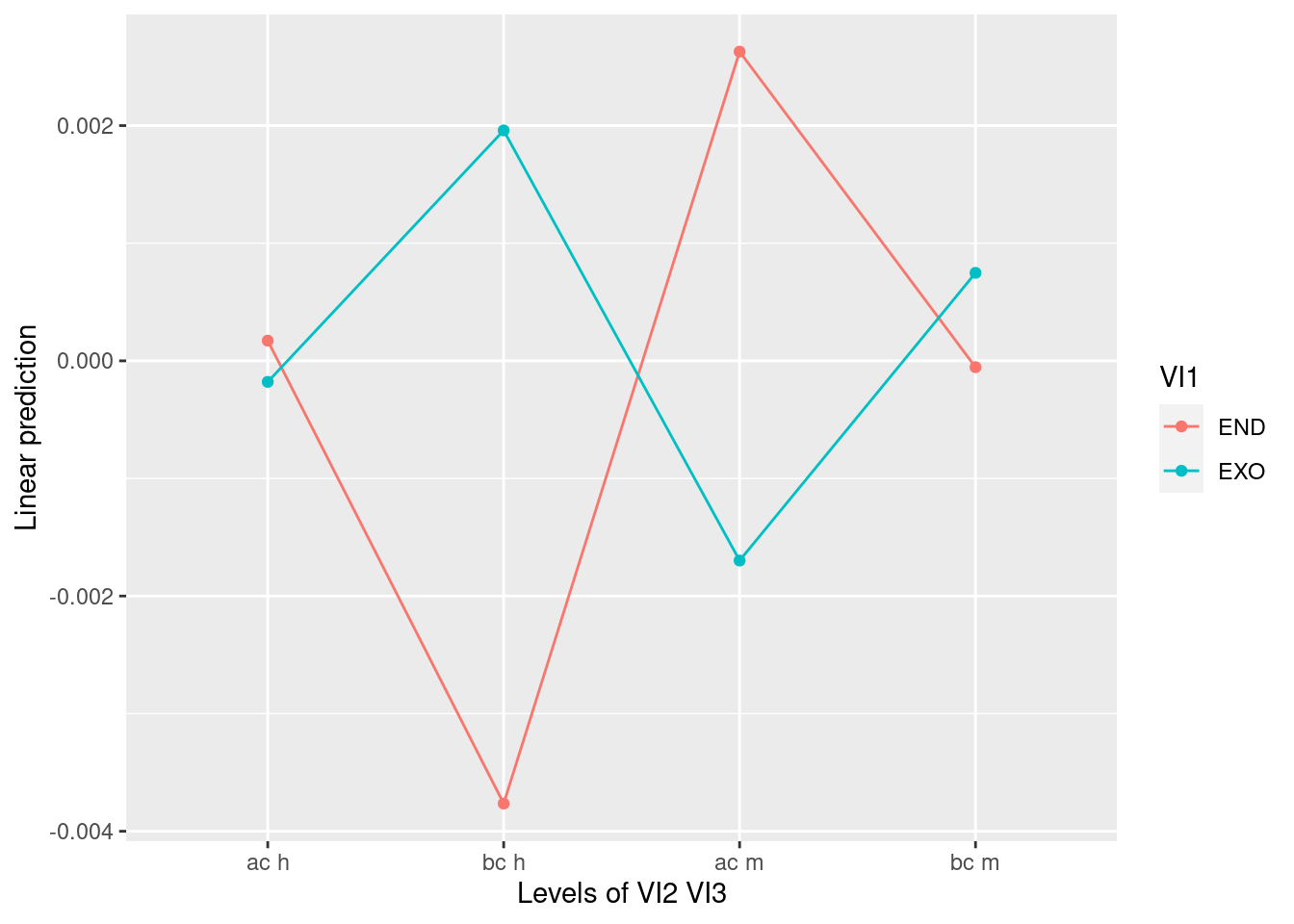

pirateplot(VD ~ VI1 * VI2 * VI3, datos_long)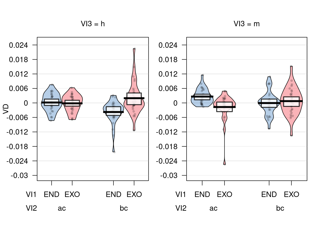

Post-hocs

lsmeans(a, c("VI1", "VI2", "VI3"), contr = "pairwise")

## $lsmeans
##  VI1 VI2 VI3    lsmean       SE  df  lower.CL  upper.CL
##  END ac  h    1.71e-04 0.000912 137 -0.001632  0.001975
##  EXO ac  h   -1.79e-04 0.000912 137 -0.001982  0.001625
##  END bc  h   -3.76e-03 0.000912 137 -0.005568 -0.001961
##  EXO bc  h    1.96e-03 0.000912 137  0.000155  0.003762
##  END ac  m    2.63e-03 0.000912 137  0.000825  0.004432
##  EXO ac  m   -1.70e-03 0.000912 137 -0.003502  0.000105
##  END bc  m   -5.43e-05 0.000912 137 -0.001858  0.001749
##  EXO bc  m    7.48e-04 0.000912 137 -0.001056  0.002551
## 
## Warning: EMMs are biased unless design is perfectly balanced 
## Confidence level used: 0.95 
## 
## $contrasts
##  contrast             estimate      SE    df t.ratio p.value
##  END ac h - EXO ac h  0.000350 0.00131  73.4  0.268  1.0000 
##  END ac h - END bc h  0.003936 0.00136  66.2  2.900  0.0890 
##  END ac h - EXO bc h -0.001787 0.00135  68.8 -1.328  0.8850 
##  END ac h - END ac m -0.002457 0.00119  69.2 -2.064  0.4479 
##  END ac h - EXO ac m  0.001870 0.00124  70.7  1.510  0.7996 
##  END ac h - END bc m  0.000226 0.00171 108.7  0.132  1.0000 
##  END ac h - EXO bc m -0.000576 0.00130  69.8 -0.442  0.9998 
##  EXO ac h - END bc h  0.003586 0.00135  68.8  2.664  0.1517 
##  EXO ac h - EXO bc h -0.002138 0.00136  66.2 -1.575  0.7631 
##  EXO ac h - END ac m -0.002808 0.00124  70.7 -2.268  0.3259 
##  EXO ac h - EXO ac m  0.001519 0.00119  69.2  1.276  0.9045 
##  EXO ac h - END bc m -0.000125 0.00130  69.8 -0.096  1.0000 
##  EXO ac h - EXO bc m -0.000927 0.00171 108.7 -0.541  0.9994 
##  END bc h - EXO bc h -0.005723 0.00131  73.4 -4.371  0.0010 
##  END bc h - END ac m -0.006393 0.00171 108.7 -3.731  0.0071 
##  END bc h - EXO ac m -0.002066 0.00130  69.8 -1.586  0.7570 
##  END bc h - END bc m -0.003710 0.00119  69.2 -3.117  0.0512 
##  END bc h - EXO bc m -0.004512 0.00124  70.7 -3.644  0.0113 
##  EXO bc h - END ac m -0.000670 0.00130  69.8 -0.514  0.9996 
##  EXO bc h - EXO ac m  0.003657 0.00171 108.7  2.134  0.4000 
##  EXO bc h - END bc m  0.002013 0.00124  70.7  1.626  0.7332 
##  EXO bc h - EXO bc m  0.001211 0.00119  69.2  1.017  0.9703 
##  END ac m - EXO ac m  0.004327 0.00131  73.4  3.305  0.0302 
##  END ac m - END bc m  0.002683 0.00136  66.2  1.977  0.5049 
##  END ac m - EXO bc m  0.001881 0.00135  68.8  1.397  0.8553 
##  EXO ac m - END bc m -0.001644 0.00135  68.8 -1.221  0.9228 
##  EXO ac m - EXO bc m -0.002446 0.00136  66.2 -1.802  0.6209 
##  END bc m - EXO bc m -0.000802 0.00131  73.4 -0.613  0.9986 
## 
## P value adjustment: tukey method for comparing a family of 8 estimates

lsmeans(a, "VI1", contr = "pairwise")

## NOTE: Results may be misleading due to involvement in interactions

## $lsmeans
##  VI1    lsmean      SE   df  lower.CL upper.CL
##  END -0.000255 0.00024 53.4 -0.000735 0.000226
##  EXO  0.000207 0.00024 53.4 -0.000273 0.000688
## 
## Results are averaged over the levels of: VI2, VI3 
## Warning: EMMs are biased unless design is perfectly balanced 
## Confidence level used: 0.95 
## 
## $contrasts
##  contrast   estimate       SE df t.ratio p.value
##  END - EXO -0.000462 0.000375 28 -1.233  0.2277 
## 
## Results are averaged over the levels of: VI2, VI3

lsmeans(a, "VI2", contr = "pairwise")

## NOTE: Results may be misleading due to involvement in interactions

## $lsmeans
##  VI2    lsmean       SE   df  lower.CL upper.CL
##  ac   0.000231 0.000499 33.5 -0.000783 0.001245
##  bc  -0.000278 0.000499 33.5 -0.001292 0.000736
## 
## Results are averaged over the levels of: VI1, VI3 
## Warning: EMMs are biased unless design is perfectly balanced 
## Confidence level used: 0.95 
## 
## $contrasts
##  contrast estimate       SE df t.ratio p.value
##  ac - bc  0.000509 0.000952 28 0.535   0.5971 
## 
## Results are averaged over the levels of: VI1, VI3

lsmeans(a, "VI3", contr = "pairwise")

## NOTE: Results may be misleading due to involvement in interactions

## $lsmeans
##  VI3    lsmean       SE   df  lower.CL upper.CL
##  h   -0.000453 0.000401 36.8 -0.001266 0.000359
##  m    0.000406 0.000401 36.8 -0.000407 0.001219
## 
## Results are averaged over the levels of: VI1, VI2 
## Warning: EMMs are biased unless design is perfectly balanced 
## Confidence level used: 0.95 
## 
## $contrasts
##  contrast  estimate       SE df t.ratio p.value
##  h - m    -0.000859 0.000744 28 -1.154  0.2581 
## 
## Results are averaged over the levels of: VI1, VI2

10.4 Mixed Models

VER NOTAS EN: “R_Statistics_Manual/NOT_FOR_GITHUB/Specific tests/lme4/GLMER Notes.md”

Ejemplo analisis en: /home/emrys/gorkang@gmail.com/RESEARCH/PROYECTOS/A1-1_WRITING/Lorena - David - Gorka/Analisis de datos - Lorena - PAPER 2/dev/analisis-finales_DEV.R

10.4.1 Reading list

https://ademos.people.uic.edu/Chapter17.html

Contrast coding:

General:

Other

http://mfviz.com/hierarchical-models/

10.5 Meta analysis

Code adapted from an example sent by Miro on 20170509

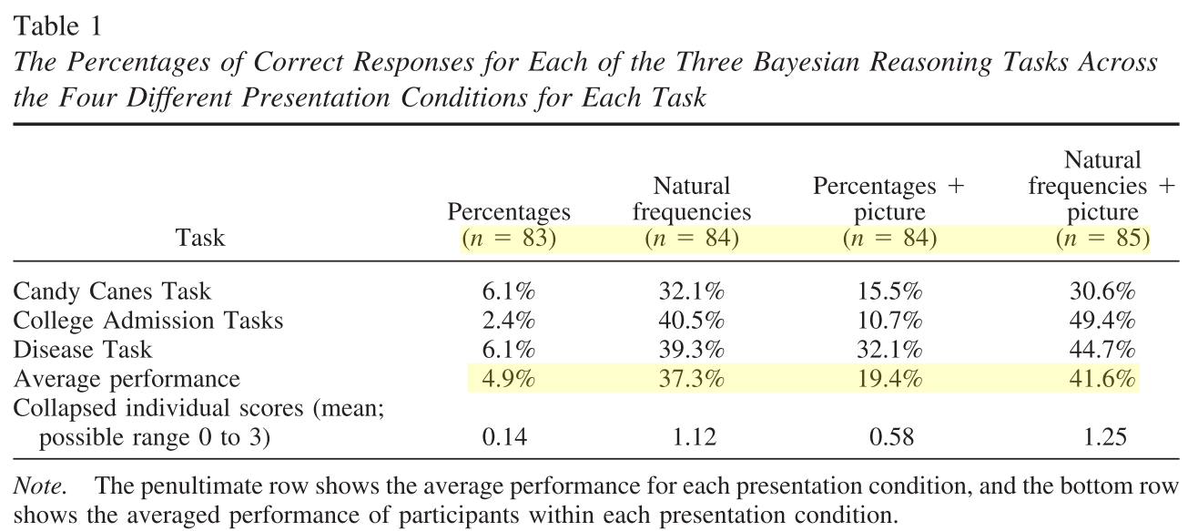
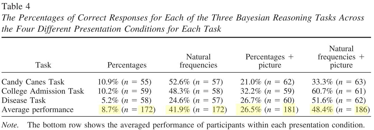
Meta-analysis of Brase, G. L., & Hill, W. T. (2017). Adding up to good Bayesian reasoning: Problem format manipulations and individual skill differences. Journal of Experimental Psychology: General, 146(4), 577–591. http://doi.org/10.1037/xge0000280

Factorial 2x2 design (aggreagted data from Experiment1 & Experiment2)

IV1: Representation format (Natural Frequencies x Probabilities)
IV2: Pictorial aid (No pictorial aid x Pictorial aid)

Experiment1

Experiment2

Libraries

if (!require('metafor')) install.packages('metafor'); library('metafor')

10.5.1 Natural Frequencies Effect

# input of the data from the two experiments, each is featuring two comparison (note: ai to di are corresponding to the 2x2 table, n1i and n2i are row sums)

Contrast = "NF - Perc"
Comparisons = c("Exp 1a No Picture", "Exp 1b Picture", "Exp 2a No Picture","Exp 2b Picture")

# NF with and without pictures
# E1_NF, E1_NF+Pic, E2_NF, E2_NF+Pic
# (84*.373, 85*.416, 172*.419, 186*.484)
ai <-  c(31, 35, 72, 90)
n1i <- c(84, 85, 172, 186)
bi <- n1i- ai # c(53, 50, 100, 96)

# Prob with and without pictures
# E1_Perc, E1_Perc+Pic, E2_Perc, E2_Perc+Pic
# (83*.049, 84*.194, 172*.087, 181*.265)
ci <- c(4, 16, 15, 48)
n2i <- c(83, 84, 172, 181)
di <- n2i - ci # di <- c(79, 68, 157, 133)

# mod <- c(0, 1, 0, 1)

# fit the fixed model and return its value for OR
rma.overallOR <- rma.uni(ai=ai, bi=bi, ci=ci, di=di, n1i=n1i, n2i=n2i, measure="OR", 
                         method="REML", weighted=TRUE,
                         level=95, digits=3)

summary(rma.overallOR)

## 
## Random-Effects Model (k = 4; tau^2 estimator: REML)
## 
##   logLik  deviance       AIC       BIC      AICc 
##   -3.205     6.410    10.410     8.607    22.410   
## 
## tau^2 (estimated amount of total heterogeneity): 0.339 (SE = 0.382)
## tau (square root of estimated tau^2 value):      0.583
## I^2 (total heterogeneity / total variability):   75.66%
## H^2 (total variability / sampling variability):  4.11
## 
## Test for Heterogeneity:
## Q(df = 3) = 12.128, p-val = 0.007
## 
## Model Results:
## 
## estimate     se   zval   pval  ci.lb  ci.ub 
##    1.542  0.342  4.507  <.001  0.871  2.213  *** 
## 
## ---
## Signif. codes:  0 '***' 0.001 '**' 0.01 '*' 0.05 '.' 0.1 ' ' 1

# rma.overallOR

forest(rma.overallOR, 
       showweight = TRUE,
       slab=Comparisons, 
       xlab="Log Odds Ratio", mlab="FE Model for All Comparisons", main = Contrast )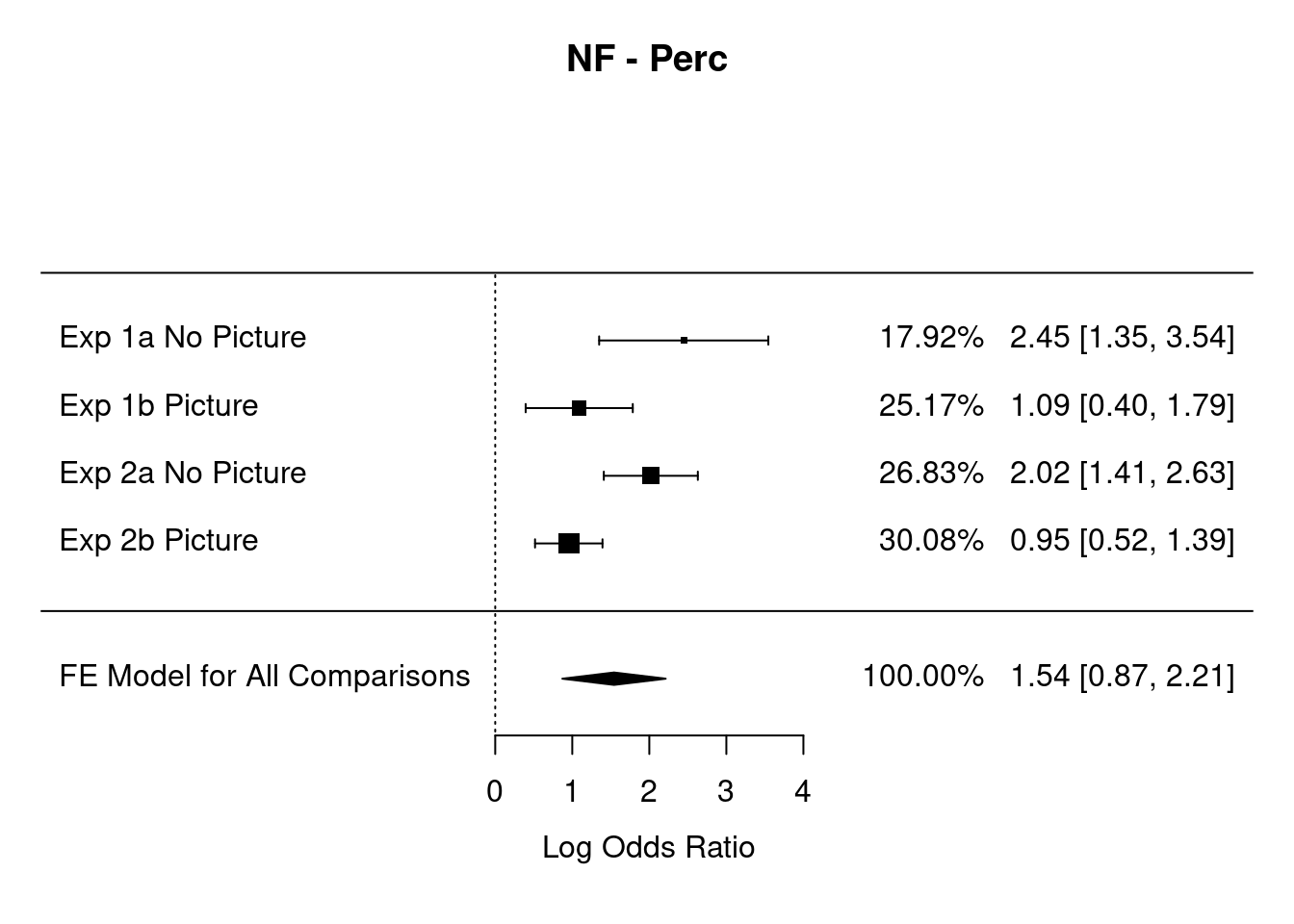

10.5.2 Pictures Effect

# input of the data from the two experiments, each is featuring two comparison (note: ai to di are corresponding to the 2x2 table, n1i and n2i are row sums)
# Here we use the parameter mod to assess moderation (???)

Contrast = "Pictures - No pictures"
Comparisons = c("Exp 1a Perc", "Exp 1b NF", "Exp 2a Perc","Exp 2b NF")


# Prob and  NF with Pictures
# E1_Perc+Pic, E1_NF+Pic, E2_Perc+Pic, E2_NF+Pic
# (84*.194,   85*.416,  181*.265, 186*.484)
ai <-  c(16, 35, 48, 90)
n1i <- c(84, 85, 181, 186)
bi <- n1i- ai # bi <- c(68, 50, 133, 96)

# Prob and  NF without Pictures
# E1_Perc, E1_NF, E2_Perc , E2_NF
# (83*.049,   84*.373,  172*.087, 172*.419)
ci <- c(4, 31, 15, 72)
n2i <- c(83, 84, 172, 172)
di <- n2i - ci # di <- c(79, 53, 157, 100)


mod <- c(0, 1, 0, 1)

# fit the fixed model and return its value for OR
  # Here we use the moderator mod
rma.overallOR <- rma.uni(ai=ai, bi=bi, ci=ci, di=di, n1i=n1i, n2i=n2i, mod=mod, measure="OR", 
                         method="REML", weighted=T,
                         level=95, digits=3)

summary(rma.overallOR)

## 
## Mixed-Effects Model (k = 4; tau^2 estimator: REML)
## 
##   logLik  deviance       AIC       BIC      AICc 
##    0.156    -0.313     5.687     1.767    29.687   
## 
## tau^2 (estimated amount of residual heterogeneity):     0 (SE = 0.097)
## tau (square root of estimated tau^2 value):             0
## I^2 (residual heterogeneity / unaccounted variability): 0.00%
## H^2 (unaccounted variability / sampling variability):   1.00
## R^2 (amount of heterogeneity accounted for):            100.00%
## 
## Test for Residual Heterogeneity:
## QE(df = 2) = 0.146, p-val = 0.929
## 
## Test of Moderators (coefficient 2):
## QM(df = 1) = 11.872, p-val < .001
## 
## Model Results:
## 
##          estimate     se    zval   pval   ci.lb   ci.ub 
## intrcpt     1.377  0.279   4.926  <.001   0.829   1.924  *** 
## mods       -1.139  0.331  -3.446  <.001  -1.787  -0.491  *** 
## 
## ---
## Signif. codes:  0 '***' 0.001 '**' 0.01 '*' 0.05 '.' 0.1 ' ' 1

# rma.overallOR

forest(rma.overallOR, 
       showweight = TRUE,
       slab= Comparisons, 
       xlab="Log Odds Ratio", mlab="REML Model for All Comparisons", main = Contrast)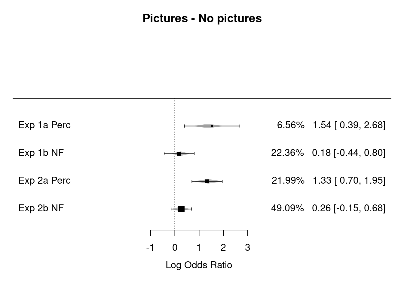

10.5.3 Notes on Meta-analysis

http://www.nicebread.de/meta-showdown-1/

10.6 ROC Curves

Code from https://github.com/dariyasydykova/tidyroc README

tidyroc won’t be developed further. It seems https://github.com/tidymodels/yardstick does everything tidyroc does and more?

Intro about what ROC curves measure: https://twitter.com/cecilejanssens/status/1104134423673479169?s=03

Why ROC curves are misleading: http://www.fharrell.com/post/mlconfusion/ (Not useful for prediction. PPV/NPV better).

if (!require('tidyroc')) remotes::install_github("dariyasydykova/tidyroc"); library('tidyroc')
# remotes::install_github("dariyasydykova/tidyroc")

  library(dplyr)
  library(ggplot2)
  library(broom)
  library(tidyroc)

  glm(am ~ disp,
      family = binomial,
      data = mtcars
  ) %>%
    augment() %>%
    make_roc(predictor = .fitted, known_class = am) %>%
    ggplot(aes(x = fpr, y = tpr)) +
    geom_line() +
    theme_minimal()

  # load tidyverse packages
  library(dplyr)
  library(ggplot2)
  library(broom)

  # load cowplot to change plot theme
  library(cowplot)

  # load tidyroc
  library(tidyroc)


  # get `biopsy` dataset from `MASS`
  data(biopsy, package = "MASS")

  # change column names from `V1`, `V2`, etc. to informative variable names
  colnames(biopsy) <-
    c("ID",
      "clump_thickness",
      "uniform_cell_size",
      "uniform_cell_shape",
      "marg_adhesion",
      "epithelial_cell_size",
      "bare_nuclei",
      "bland_chromatin",
      "normal_nucleoli",
      "mitoses",
      "outcome")

  # fit a logistic regression model to predict tumor types
  glm_out1 <- glm(
    formula = outcome ~ clump_thickness + uniform_cell_shape + marg_adhesion + bare_nuclei + bland_chromatin + normal_nucleoli,
    family = binomial,
    data = biopsy
  ) %>%
    augment() %>%
    mutate(model = "m1") # name the model

  # fit a different logistic regression model to predict tumor types
  glm_out2 <- glm(outcome ~ clump_thickness,
                  family = binomial,
                  data = biopsy
  ) %>%
    augment() %>%
    mutate(model = "m2") # name the model

  # combine the two datasets to make an ROC curve for each model
  glm_out <- bind_rows(glm_out1, glm_out2)

  # plot the distribution of fitted values to see both models' outcomes
  glm_out %>%
    ggplot(aes(x = .fitted, fill = outcome)) +
    geom_density(alpha = 0.6, color = NA) +
    scale_fill_manual(values = c("#F08A5D", "#B83B5E")) +
    facet_wrap(~ model)


  # plot ROC curves
  glm_out %>%
    group_by(model) %>% # group to get individual ROC curve for each model
    make_roc(predictor = .fitted, known_class = outcome) %>% # get values to plot an ROC curve
    ggplot(aes(x = fpr, y = tpr, color = model)) +
    geom_line(size = 1.1) +
    geom_abline(slope = 1, intercept = 0, size = 0.4) +
    scale_color_manual(values = c("#48466D", "#3D84A8")) +
    theme_cowplot()


  # plot precision-recall curves using the data-frame we generated in the previous example
  glm_out %>%
    group_by(model) %>% # group to get individual precision-recall curve for each model
    make_pr(predictor = .fitted, known_class = outcome) %>% # get values to plot a precision-recall curve
    ggplot(aes(x = recall, y = precision, color = model)) +
    geom_line(size = 1.1) +
    coord_cartesian(ylim = c(0, 1), xlim = c(0, 1)) +
    scale_color_manual(values = c("#48466D", "#3D84A8")) +
    theme_cowplot()

  glm_out %>%
    group_by(model) %>% # group to get individual AUC values for each ROC curve
    make_roc(predictor = .fitted, known_class = outcome) %>%
    summarise(auc = calc_auc(x = fpr, y = tpr))

  ## # A tibble: 2 x 2
  ##   model   auc
  ##   <chr> <dbl>
  ## 1 m1    0.996
  ## 2 m2    0.910

  glm_out %>%
    group_by(model) %>% # group to get individual AUC values for each precision-recall curve
    make_pr(predictor = .fitted, known_class = outcome) %>%
    summarise(auc = calc_auc(x = recall, y = precision))

  ## # A tibble: 2 x 2
  ##   model   auc
  ##   <chr> <dbl>
  ## 1 m1    0.991
  ## 2 m2    0.951

Leys, C., Ley, C., Klein, O., Bernard, P. & Licata, L. Detecting outliers: Do not use standard deviation around the mean, use absolute deviation around the median. J. Exp. Soc. Psychol. 49, 764–766 (2013).↩︎
See Serban C. Musca post ↩︎

10 Estadistica inferencial

10.1 Referencias y Fuentes

10.2 Association test

10.2.1 Frequentist1

10.2.2 Bayesian2

10.2.3 Results report - WIP

10.2.3.1 Frequentist - WIP

10.2.3.2 Bayesian

10.2.4 References

10.3 ANOVA repeated measures

10.4 Mixed Models

10.4.1 Reading list

10.5 Meta analysis

10.5.1 Natural Frequencies Effect

10.5.2 Pictures Effect

10.5.3 Notes on Meta-analysis

10.6 ROC Curves

10.2.1 Frequentist¹

10.2.2 Bayesian²