8 Visualizar riesgo
8.1 Riskr
FROM: https://cran.r-project.org/web/packages/riskyr/vignettes/E_riskyr_primer.html
if (!require('riskyr')) install.packages('riskyr'); library('riskyr')

# Create a customized scenario:
my.scenario <- riskyr(scen_lbl = "Identifying reoffenders",
                      popu_lbl = "prison inmates",
                      cond_lbl = "reoffending",
                      cond_true_lbl = "offends again", cond_false_lbl = "does not offend again",
                      dec_lbl = "test result",
                      dec_pos_lbl = "predict to\nreoffend", dec_neg_lbl = "predict to\nnot reoffend",
                      hi_lbl = "reoffender found", mi_lbl = "reoffender missed",
                      fa_lbl = "false accusation", cr_lbl = "correct release",
                      prev = .45,  # prevalence of being a reoffender.
                      sens = .98,  # p( will reoffend | offends again )
                      spec = .46,  # p( will not reoffend | does not offend again )
                      fart =  NA,  # p( will reoffend | does not offend gain )
                      N = 753,     # population size
                      scen_src = "(a ficticious example)")


my.scenario <- scenarios$n6

summary(my.scenario)
## Scenario: Mammography (prob)
##
## Condition: Breast cancer
## Decision: Screening
## Population: Women (age 40)
## N = 1000
## Source: Hoffrage et al. (2015), p. 3
##
## Probabilities:
##
## Essential probabilities:
## prev sens mirt spec fart
## 0.010 0.800 0.200 0.904 0.096
##
## Other probabilities:
## ppod PPV NPV FDR FOR acc
## 0.103 0.078 0.998 0.922 0.002 0.903
##
## Frequencies:
##
## by conditions:
## cond_true cond_false
## 10 990
##
## by decision:
## dec_pos dec_neg
## 103 897
##
## by correspondence (of decision to condition):
## dec_cor dec_err
## 903 97
##
## 4 essential (SDT) frequencies:
## hi mi fa cr
## 8 2 95 895
##
## Accuracy:
##
## acc:
## 0.90296plot(my.scenario, plot.type = "icons")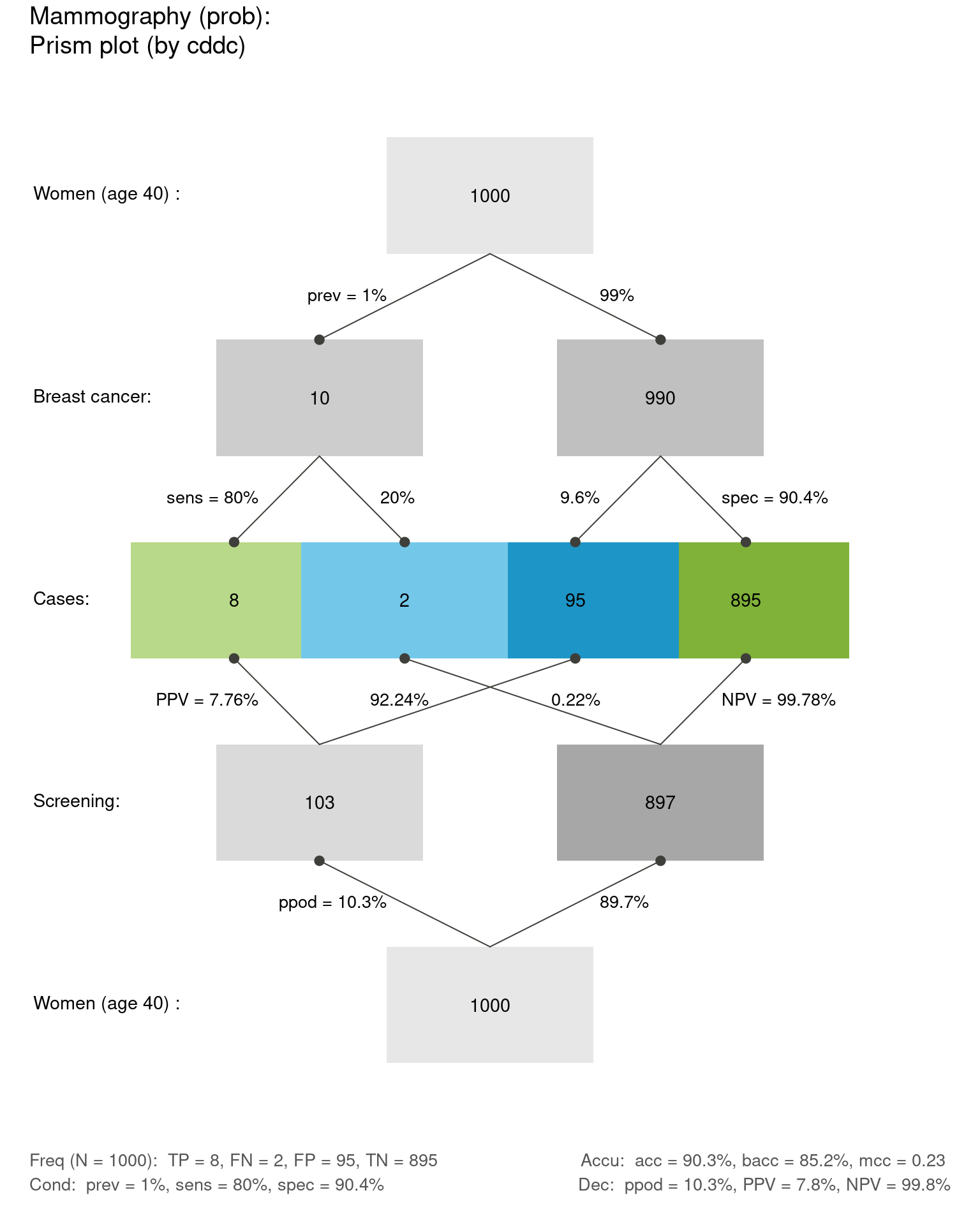
plot(my.scenario, plot.type = "tree", by = "dc") # plot tree diagram (splitting N by decision)
plot(my.scenario, plot.type = "curve") # plot default curve [what = c("prev", "PPV", "NPV")]:
if (!require('riskyr')) install.packages('riskyr'); library('riskyr')

# Use a predefined scenario
my.scenario <- scenarios$n6

summary(my.scenario)
## Scenario: Mammography (prob)
##
## Condition: Breast cancer
## Decision: Screening
## Population: Women (age 40)
## N = 1000
## Source: Hoffrage et al. (2015), p. 3
##
## Probabilities:
##
## Essential probabilities:
## prev sens mirt spec fart
## 0.010 0.800 0.200 0.904 0.096
##
## Other probabilities:
## ppod PPV NPV FDR FOR acc
## 0.103 0.078 0.998 0.922 0.002 0.903
##
## Frequencies:
##
## by conditions:
## cond_true cond_false
## 10 990
##
## by decision:
## dec_pos dec_neg
## 103 897
##
## by correspondence (of decision to condition):
## dec_cor dec_err
## 903 97
##
## 4 essential (SDT) frequencies:
## hi mi fa cr
## 8 2 95 895
##
## Accuracy:
##
## acc:
## 0.90296plot(my.scenario, plot.type = "icons")
plot(my.scenario, plot.type = "tree", by = "dc") # plot tree diagram (splitting N by decision)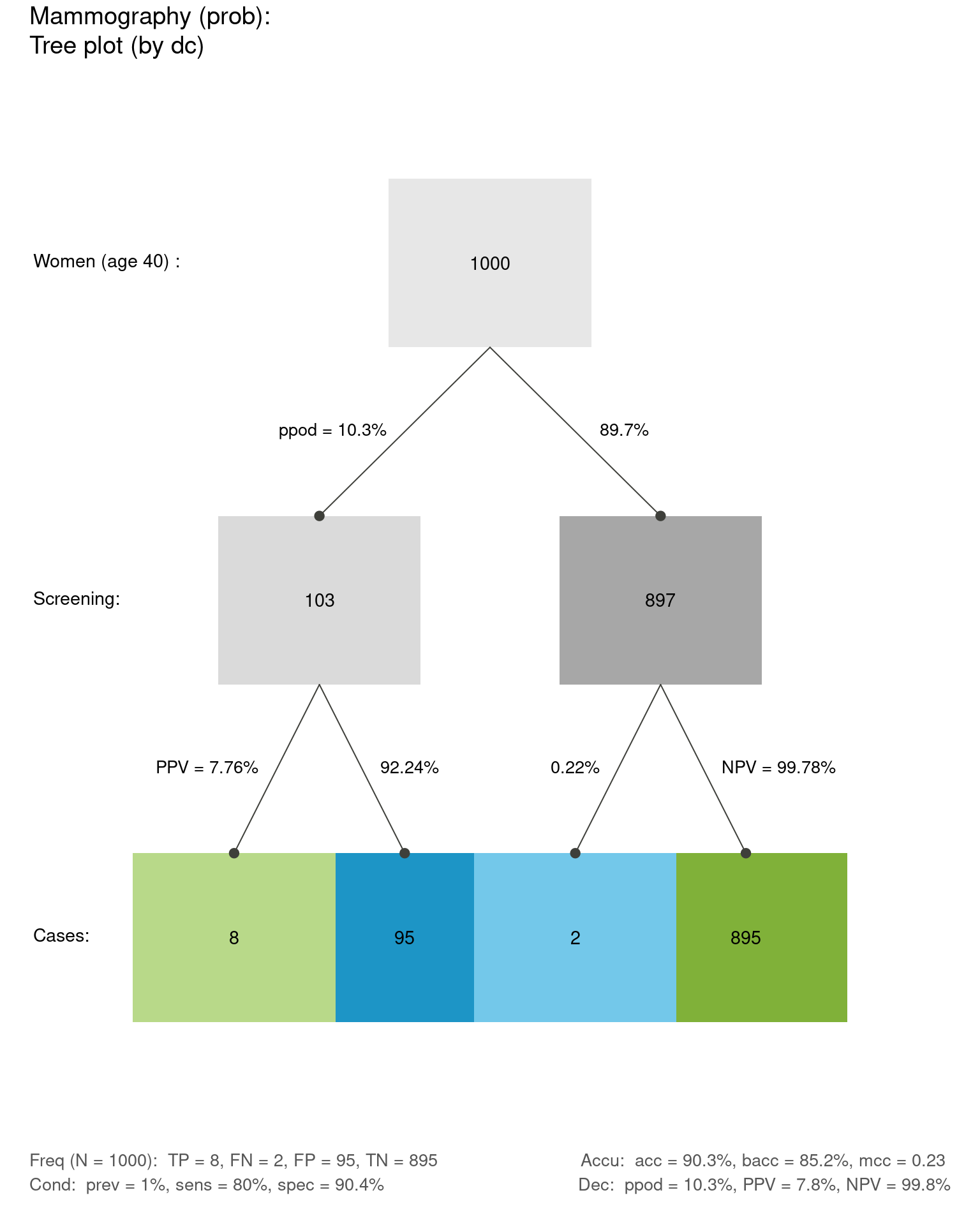
plot(my.scenario, plot.type = "curve") # plot default curve [what = c("prev", "PPV", "NPV")]:
plot(my.scenario, plot.type = "fnet", area = "sq") # network diagram (with numeric probability labels):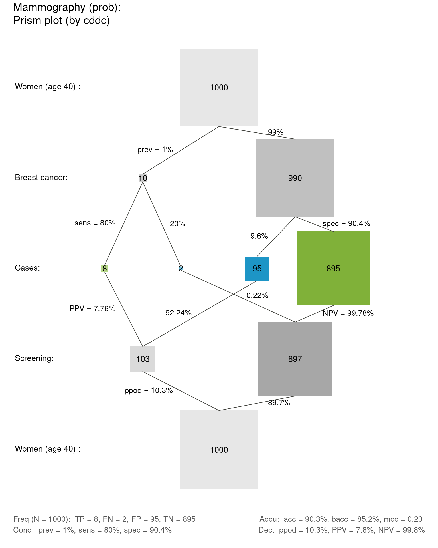
plot(my.scenario, plot.type = "curve", what = "all") # plot "all" available curves: