13 Experimental design

13.1 Tamaño de muestra y efecto detectado

En esta simulación se muestra como con tamaños de muestra pequeños, se sobreestima el tamaño de efecto real. Como se puede ver en el codigo, solo se muestran los estudios simulados donde la correlacion es significativa. Ver el blog de Jim Grange para una explicación más detallada.

# https://jimgrange.wordpress.com/2017/03/06/low-power-effect-sizes/
#------------------------------------------------------------------------------
rm(list = ls())

set.seed(50)

# function for generating random draws from multivariate distribution
# n = number of draws; p = number of variables
# u = mean of each variable; s = SD of each variable
# corMat = correlation matrix
mvrnorm <- function(n, p, u, s, corMat) {
  Z <- matrix(rnorm(n * p), p, n)
  t(u + s * t(chol(corMat)) %*% Z)
}

#------------------------------------------------------------------------------

#------------------------------------------------------------------------------
### simulation setup

# declare simulation parameters
means <- c(100, 600)
sds <- c(20, 80)
n_sims = 1000

# declare correlation coefficient & generate cor. matrix
cor <- 0.3
cor_mat <- matrix(c(1, cor, 
                    cor, 1), nrow = 2, ncol = 2, byrow = TRUE)

# sample sizes to simulate
sample_sizes <- c(10, 20, 30, 50, 85, 170, 500, 1000)

# number of simulations

# create variable to store data in
final_data <- matrix(nrow = n_sims, ncol = length(sample_sizes))
colnames(final_data) <- sample_sizes
#------------------------------------------------------------------------------

#------------------------------------------------------------------------------
### simulation execution

for(i in 1:length(sample_sizes)){
  for(j in 1:n_sims){
    
    # get the experiment data
    sim_data <- mvrnorm(sample_sizes[i], p = 2, u = means, s = sds, 
                        corMat = cor_mat)
    
    # perform the correlation
    sim_cor <- cor.test(sim_data[, 1], sim_data[, 2], method = "pearson")
    
    # if the correlation is significant, store the effect size
    if(sim_cor$p.value < 0.05){
      final_data[j, i] <- as.numeric(round(abs(sim_cor$estimate), 3))
    }
  }
}
#------------------------------------------------------------------------------

#------------------------------------------------------------------------------
## draw the plot
boxplot(final_data, na.action=na.omit, xlab = "Simulated Sample Size", 
        ylab = "Measured Effect Size")
abline(h = cor, col = "red", lty = 2, lwd = 3)

legend("topright", "True Effect Size", cex = 1.5,  lty = 2, bty="n", 
       col = "red", lwd = 3)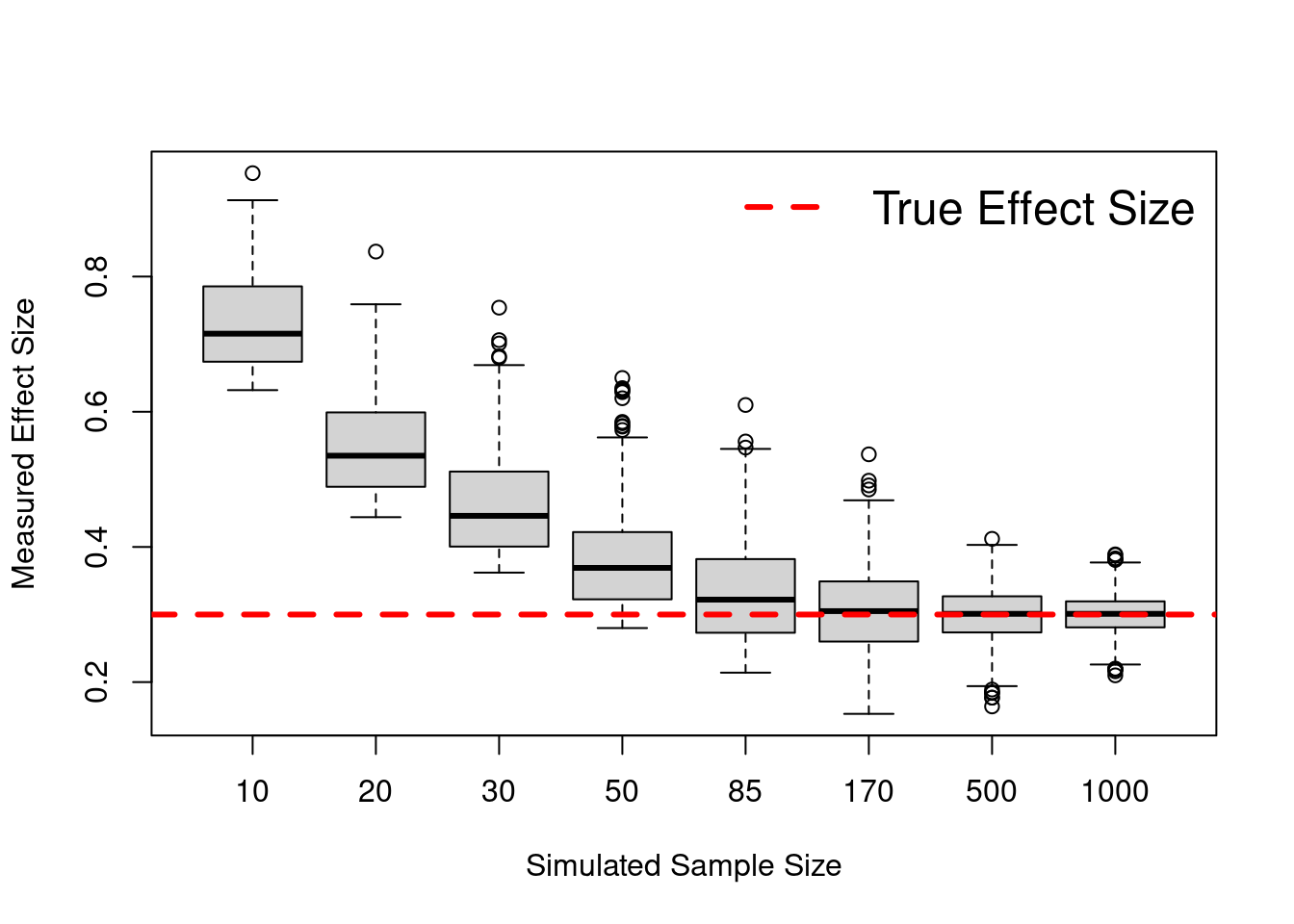

13.2 Power analysis

Usamos el paquete pwr: https://cran.r-project.org/web/packages/pwr/vignettes/pwr-vignette.html. En este tenemos un conjunto de funciones que nos permiten hacer power analysis para distintos tipos de diseños:

• pwr.p.test: one-sample proportion test
• pwr.2p.test: two-sample proportion test
• pwr.2p2n.test: two-sample proportion test (unequal sample sizes)
• vpwr.t.test: two-sample, one-sample and paired t-tests
• pwr.t2n.test: two-sample t-tests (unequal sample sizes)
• pwr.anova.test: one-way balanced ANOVA
• pwr.r.test: correlation test
• pwr.chisq.test: chi-squared test (goodness of fit and association)
• pwr.f2.test: test for the general linear model

En cada uno de ellos podemos modificar varios parámetros. El parámetro que dejemos sin especificar será el que se calculará:

• k = groups
  
• n = participants (in each group)
  
• f = effect size
  
• sig.level = sig level
  
• power = power
  
• etc.

Conventional effect sizes for all tests in the pwr package (SOURCE: https://cran.r-project.org/web/packages/pwr/vignettes/pwr-vignette.html):

Test	small	medium	large
tests for proportions (p)	0.2	0.5	0.8
tests for means (t)	0.2	0.5	0.8
chi-square tests (chisq)	0.1	0.3	0.5
correlation test (r)	0.1	0.3	0.5
anova (anov)	0.1	0.25	0.4
general linear model (f2)	0.02	0.15	0.35

Libraries

if (!require('pwr')) install.packages('pwr'); library('pwr')

Code

#T-test
pwr.t.test(n = , d = 0.8, sig.level = 0.05, power = 0.95, type = c("two.sample"))

## 
##      Two-sample t test power calculation 
## 
##               n = 41.59413
##               d = 0.8
##       sig.level = 0.05
##           power = 0.95
##     alternative = two.sided
## 
## NOTE: n is number in *each* group

#T-test 
pwr.t2n.test(n1 = 150, n2 = 75, d = , sig.level = 0.05, power = 0.8)

## 
##      t test power calculation 
## 
##              n1 = 150
##              n2 = 75
##               d = 0.3979226
##       sig.level = 0.05
##           power = 0.8
##     alternative = two.sided

#Anova 
pwr.anova.test(k = 3, n = , f = .25, sig.level = 0.05, power = .8)

## 
##      Balanced one-way analysis of variance power calculation 
## 
##               k = 3
##               n = 52.3966
##               f = 0.25
##       sig.level = 0.05
##           power = 0.8
## 
## NOTE: n is number in each group

#Effect size that we can detect
pwr.anova.test(k = 6, n = 42, sig.level = 0.05, power = .95)

## 
##      Balanced one-way analysis of variance power calculation 
## 
##               k = 6
##               n = 42
##               f = 0.283334
##       sig.level = 0.05
##           power = 0.95
## 
## NOTE: n is number in each group

#Sample size needed to detect an effect of f=0.5
pwr.anova.test(k = 2, f = 0.5, sig.level = 0.05, power = .95)

## 
##      Balanced one-way analysis of variance power calculation 
## 
##               k = 2
##               n = 26.9892
##               f = 0.5
##       sig.level = 0.05
##           power = 0.95
## 
## NOTE: n is number in each group

# General linear model
  # See example in https://cran.r-project.org/web/packages/pwr/vignettes/pwr-vignette.html
  pwr.f2.test(u = 2, f2 = 0.3/(1 - 0.3), sig.level = 0.001, power = 0.8)

## 
##      Multiple regression power calculation 
## 
##               u = 2
##               v = 49.88971
##              f2 = 0.4285714
##       sig.level = 0.001
##           power = 0.8

  #  n=v+u+1. Therefore he needs 50 + 2 + 1 = 53 student records.

13.2.1 Longitudinal designs

Calculate sample size for longitudinal designs

Libraries

if (!require('powerMediation')) install.packages('powerMediation'); library('powerMediation')

Code

ssLong(es = 0.5, #  effect size of the difference of mean change.
       rho = 0.5, # correlation coefficient between baseline and follow-up values within a treatment group.
       alpha = 0.05, 
       power = 0.95)

## [1] 104

13.3 Anonimizar participantes - Encriptar IDs

Con safer podemos encriptar cualquier cosa.

Con hashids solo podemos encriptar IDs numericos.

Libraries

if (!require('hashids')) install.packages('hashids'); library('hashids')
if (!require('safer')) install.packages('safer'); library('safer')
if (!require('dplyr')) install.packages('dplyr'); library('dplyr')

13.3.1 Encriptando y desencriptando un elemento

# No acepta acentos, ñs, etc.
h = hashid_settings(salt = 'this is my salt')

# Numbers to encode
Plain_ID = c(12345678); Plain_ID

## [1] 12345678

a = encode(Plain_ID, h); a #"BZ9RNV"

## [1] "BZ9RNV"

decode("BZ9RNV", h) #12345678

## [1] 12345678

13.3.2 Encriptando y desencriptando la columna RUT de una DB completa.

Generamos aleatoriamente numeros de identificacion “similares” a RUTs, los encriptamos, y despues desencriptamos.

# Cargamos librerias y leemos DB
if (!require('hashids')) install.packages('hashids'); library('hashids')
if (!require('dplyr')) install.packages('dplyr'); library('dplyr')

# Pseudo RUTs generadas aleatoriamente
data = round(runif(100)*10000000) %>% as_tibble() %>% 
  dplyr::rename(RUT = value)

BUG: When building book with Bookdown, it ignores the rowwise() argument!?

h = hashid_settings(salt = 'this is my salt')

# Encriptamos
data = data %>% 
  dplyr::rowwise() %>% 
  mutate(RUT_Encripted = encode(RUT, h))

# Desencriptamos
data = data %>% 
  dplyr::rowwise() %>% 
  mutate(RUT_Decripted = decode(RUT_Encripted, h))

# Mostramos los resultados
data %>% select(RUT_Encripted, RUT_Decripted, RUT)

## # A tibble: 100 x 3
## # Rowwise: 
##    RUT_Encripted RUT_Decripted     RUT
##    <chr>                 <dbl>   <dbl>
##  1 8RExa               2832261 2832261
##  2 l9aMNQ              7583306 7583306
##  3 WqOm93              3955537 3955537
##  4 xKXQoL              8587857 8587857
##  5 aporP               2879598 2879598
##  6 EOL3By              9179372 9179372
##  7 6g79nq              5208890 5208890
##  8 LK2er               1422724 1422724
##  9 jr47mN              5975451 5975451
## 10 BQ1jBQ              9688978 9688978
## # … with 90 more rows

13.3.3 Encriptando algo que no sean numeros

if (!require('safer')) install.packages('safer'); library('safer')
if (!require('dplyr')) install.packages('dplyr'); library('dplyr')

temp <- encrypt_string("hello, how are you", key = "mi clave secreta")
decrypt_string(temp, "mi clave secreta")



KEY = "my super secret key"

# Pseudo RUTs generadas aleatoriamente
data = round(runif(100)*10000000) %>% as_tibble() %>% 
  dplyr::rename(RUT = value)

# **BUG: When building book with Bookdown, it ignores the rowwise() argument!?**. Sin este argumento falla la funcion

data %>% 
  mutate(RUT = paste0("x", RUT)) %>% 
  
  # Encrypt
  rowwise() %>% 
  mutate(ID = encrypt_string(as.character(RUT), key = KEY)) %>% 
  select(RUT, ID) %>% 
  
  # Decrypt
  mutate(ID2 = decrypt_string(ID, key = KEY)) 

13.4 Match participants

---

Usaremos la siguiente Base de datos

---

# Cargamos librerias y leemos DBif (!require('pacman')) install.packages('pacman'); library('pacman')
if (!require('optmatch')) install.packages('optmatch'); library('optmatch')
if (!require('readr')) install.packages('readr'); library('readr')
if (!require('dplyr')) install.packages('dplyr'); library('dplyr')

# Archivo de data crudos
# RUTs y Edades generadas aleatoriamente
data = read_csv("Data/11-Experimental_design/Match_participants.csv")

head(data)

## # A tibble: 6 x 7
##      ID    RUT Sexo    Edad Ocupacion                 Educacion Porcentaje_ahor…
##   <dbl>  <dbl> <chr>  <dbl> <chr>                     <chr>                <dbl>
## 1     1 588006 Mujer     29 ASISTENTE DE TESORERIA    Técnica                 10
## 2     2 188576 Mujer     21 Ingeniero Comercial       Maestría                50
## 3     3 206609 Hombre    46 trabajador                Técnica                  5
## 4     4 404898 Mujer     52 Psicóloga                 Maestría                 0
## 5     5 533281 Mujer     63 Controller Postgrados Ej… Maestría                 4
## 6     6  60824 Hombre    29 Ingeniro Comercial        Maestría                 8

Preparamos la base de datos

# Umbrales para ahorradores y no ahorradores
Criterio_ahorradores = 20
Criterio_no_ahorradores = 2

# Mostramos histograma
hist(data$Porcentaje_ahorro, breaks = 100)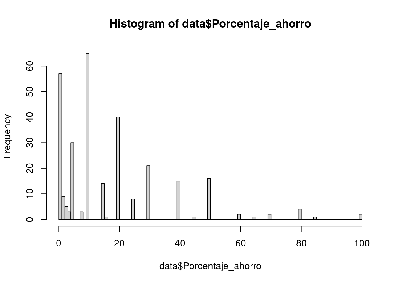

# Creamos grupos de Ahorradores (0) y No ahorradores (1)
data$Ahorro = ifelse(data$Porcentaje_ahorro <= Criterio_no_ahorradores, 1,
                      ifelse(data$Porcentaje_ahorro >= Criterio_ahorradores, 0, NA
                      ))

# Cuantos tenemos en cada grupo?
table(data$Ahorro)

## 
##   0   1 
## 113  66

#Limpiamos NAs en Ahorro y RUTs duplicados
data = data[complete.cases(data),]
data = data[!duplicated(data$ID),]

#Eliminamos a los Estudiantes
data = data[!grepl("studiante", data$Ocupacion),]

#Recreamos columna ID para los registros que quedan
data$ID = seq(1:nrow(data))

Realizamos el matching

TODO: Como evaluamos si el matching es bueno?

#Creamos base de parejas
parejas = as.data.frame((optmatch::pairmatch(Ahorro ~ Edad + Sexo + Educacion, data = data)))
    # caliper establece limites para los matchings
    # print(pairmatch(Ahorro ~ Edad + Sexo + Educacion, caliper = 4.9, data = data), grouped = TRUE)

#Como evaluamos si es buena la seleccion?
# summary(lm(Ahorro ~ Edad + Sexo + Educacion, data = data))

#Añadimos columna ID y renombramos columnas
parejas$ID = seq(1:nrow(data))
colnames(parejas) = c("Group", "ID")

#Combinamos ambas bases y limpiamos
datos_combinados = merge(data, parejas, by = "ID")
datos_combinados = datos_combinados[complete.cases(datos_combinados),]

#Ordenamos por Num de grupo y Ahorro
datos_finales = datos_combinados %>% arrange(Group, Ahorro)

#Cuantos en cada grupo?
table(datos_finales$Ahorro)

## 
##  0  1 
## 58 58

# datos_finales %>% dplyr::select(Edad, Sexo, Educacion, Porcentaje_ahorro)

13.5 Determine distribution

FROM: https://stats.stackexchange.com/questions/132652/how-to-determine-which-distribution-fits-my-data-best

Which ditribution best fits our data.

if(!require('fitdistrplus')) install.packages('fitdistrplus'); library('fitdistrplus')
if(!require('logspline')) install.packages('logspline'); library('logspline')

x <- c(37.50,46.79,48.30,46.04,43.40,39.25,38.49,49.51,40.38,36.98,40.00,
       38.49,37.74,47.92,44.53,44.91,44.91,40.00,41.51,47.92,36.98,43.40,
       42.26,41.89,38.87,43.02,39.25,40.38,42.64,36.98,44.15,44.91,43.40,
       49.81,38.87,40.00,52.45,53.13,47.92,52.45,44.91,29.54,27.13,35.60,
       45.34,43.37,54.15,42.77,42.88,44.26,27.14,39.31,24.80,16.62,30.30,
       36.39,28.60,28.53,35.84,31.10,34.55,52.65,48.81,43.42,52.49,38.00,
       38.65,34.54,37.70,38.11,43.05,29.95,32.48,24.63,35.33,41.34)
descdist(x, discrete = FALSE)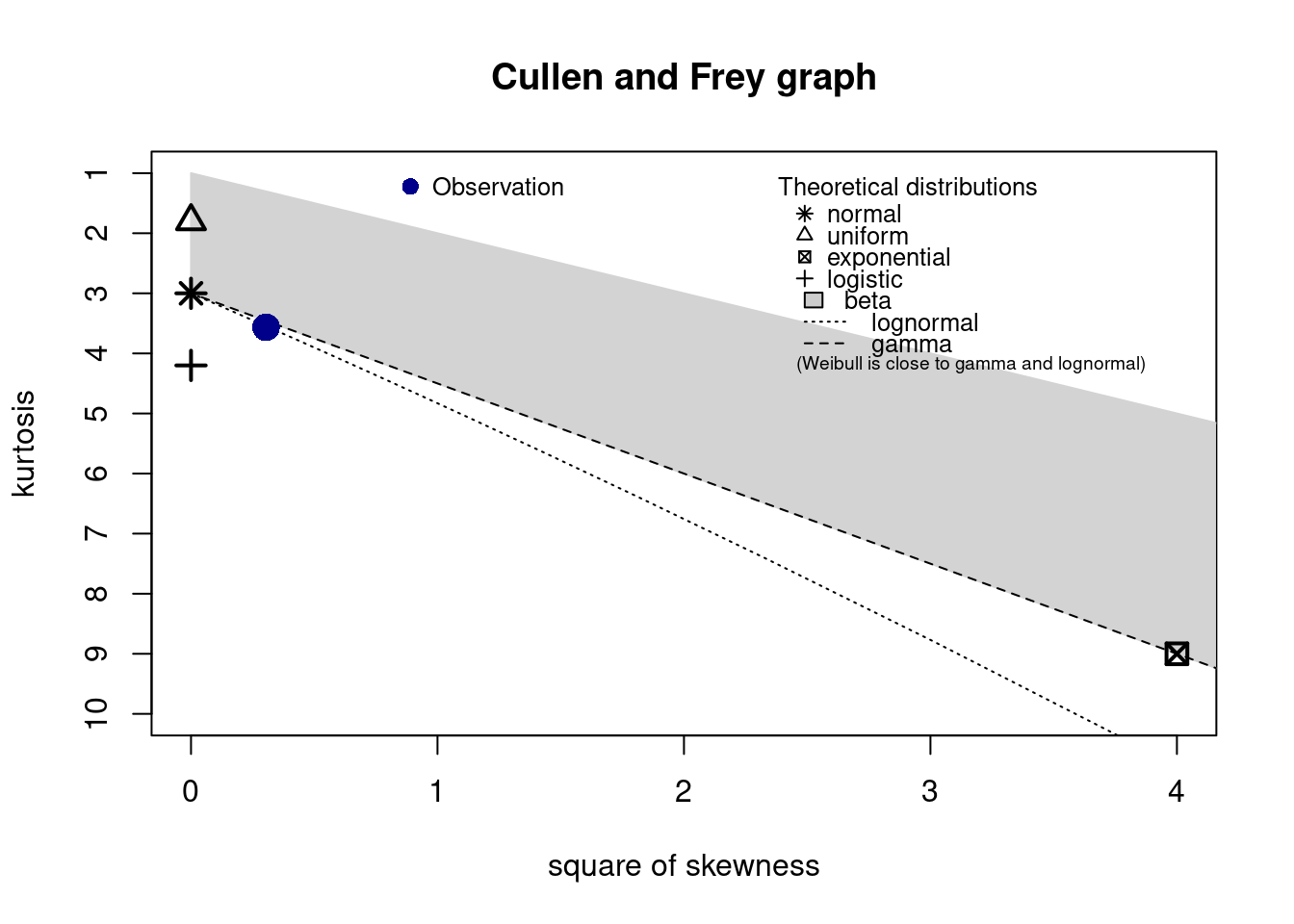

## summary statistics
## ------
## min:  16.62   max:  54.15 
## median:  40.38 
## mean:  40.28434 
## estimated sd:  7.420034 
## estimated skewness:  -0.551717 
## estimated kurtosis:  3.565162